Overview

In this project, I explore some interesting features with regards to filters and frequencies and have produced some of the very interesting results. It really hits me that the operations we see in our app are not just so simple as it seems, it actually requires a lot of thinking and implementation.

Part 1: Fun with Filters

We always start our journey with the simple convolution kernel.

$D_x = \begin{bmatrix} 1 & 0 & -1 \end{bmatrix} \quad \text{and} \quad D_y = \begin{bmatrix} 1 \\ 0 \\ -1 \end{bmatrix}$

1.1 Convolution from scratch

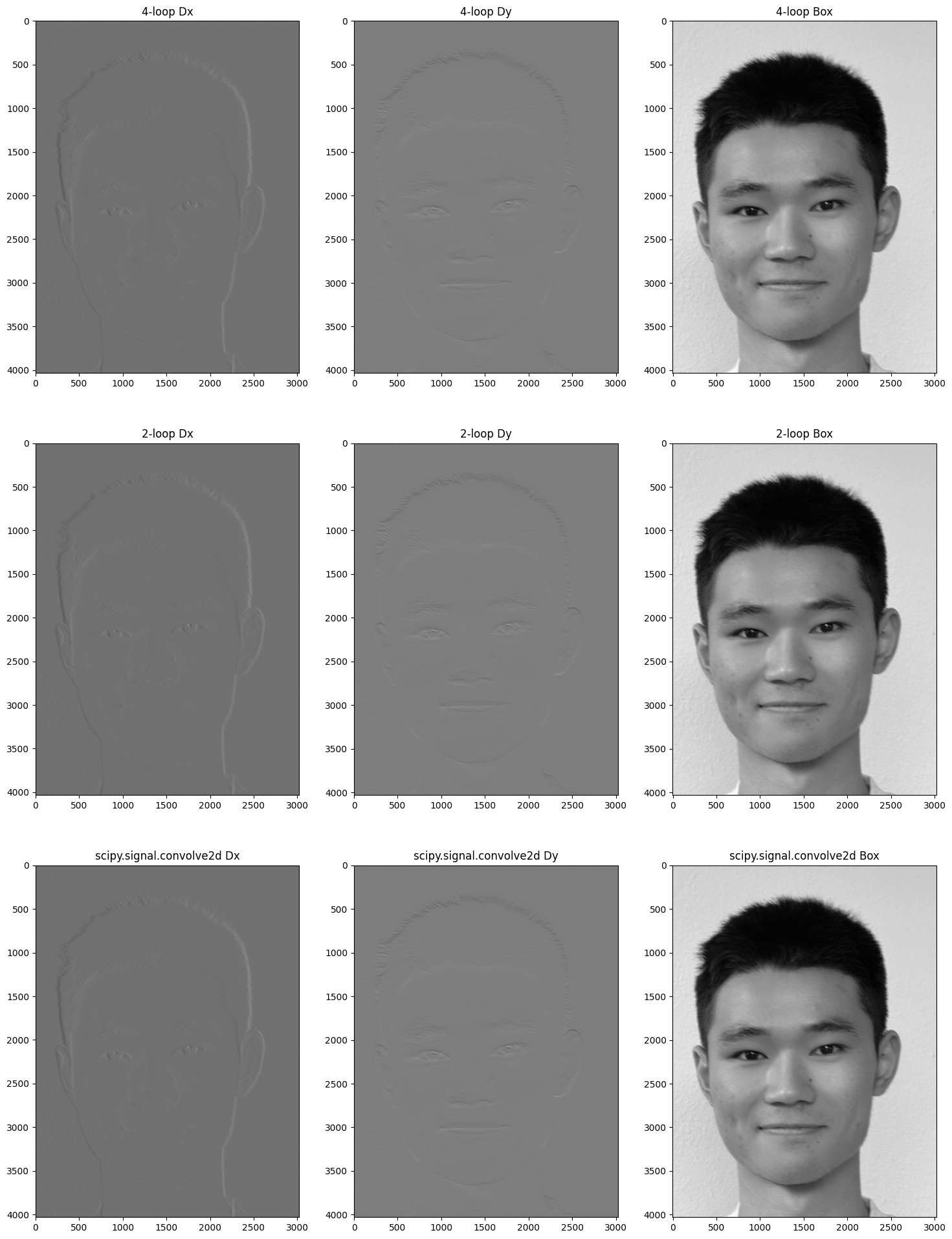
In this part, I implement the convolution using 4 loops and the 2 loops methods.

For the 4 loops method, I iterate over the output dimensions and then the kernel dimensions to calculate the sum of the product of the image and the kernel.

def conv2d_4loops(image, kernel, padding: Tuple[int, int] = (0, 0)):
    image = np.pad(image, ((padding[0], padding[0]), (padding[1], padding[1])), mode='constant')
    kernel = np.flip(kernel, axis=(0, 1))
    
    im_h, im_w = image.shape
    kh, kw = kernel.shape
    assert kh % 2 == 1 and kw % 2 == 1, "Kernel must have odd dimensions, currently {}x{}".format(kh, kw)
    
    out_h = im_h - kh + 1
    out_w = im_w - kw + 1
    output = np.zeros((out_h, out_w))
    
    for i in range(out_h):
        for j in range(out_w):
            acc = 0.0
            for m in range(kh):
                for n in range(kw):
                    ii = i + m
                    jj = j + n
                    acc += image[ii, jj] * kernel[m, n]
            output[i, j] = acc
    return output

We can observe that actually each of the kernel entry is multiplied by the image entry and then summed up, so we can first flip the kernel and use the kernel entries to multiply slice of the image. This avoids the frequent indexing of the image. Here is the implementation of the 2 loops method:

def conv2d_2loops(image, kernel, padding: Tuple[int, int] = (0, 0)):
    image = np.pad(image, ((padding[0], padding[0]), (padding[1], padding[1])), mode='constant')
    im_h, im_w = image.shape
    kh, kw = kernel.shape
    out_h = im_h - kh + 1
    out_w = im_w - kw + 1
    output = np.zeros((out_h, out_w))
    
    kernel = np.flip(kernel, axis=(0, 1))
    
    for i in range(kh):
        for j in range(kw):
            output += image[i:i+out_h, j:j+out_w] * kernel[i, j] # Key Computation
    return output

By comparing the two implementations with scipy convolution implementation, we can see that the second method is much faster.

Method	4 Loops	2 Loops	Scipy
Time (s)	187.68	1.25	2.11

1.2 Finite Difference Operator

In this part, we are trying to detect the edges of the image using the finite difference operator.

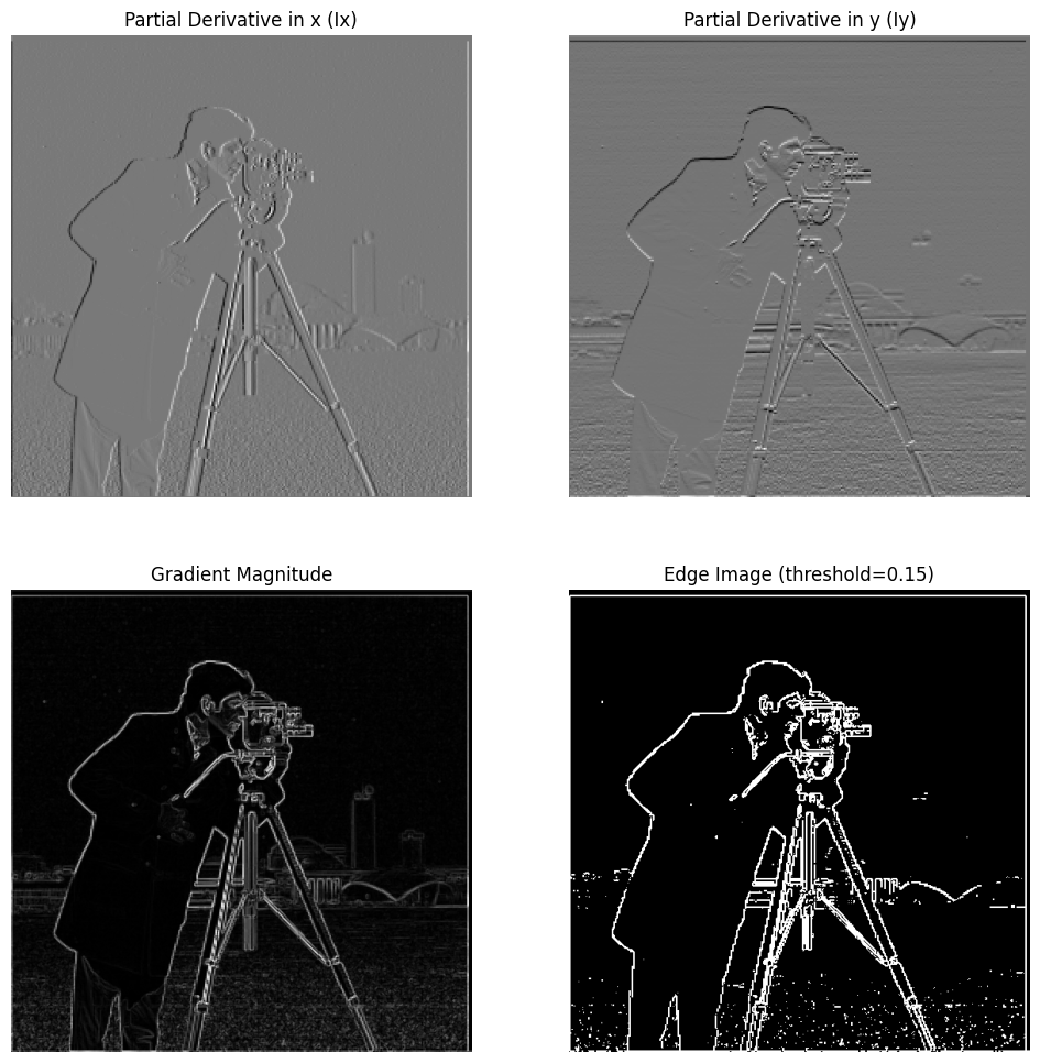
The edge detection is simply by calculating the magnitude of the gradient of the image. And then use the threshold to get the edge image. Here I choose 0.15 as the threshold.

1
2
3

grad_mag = np.sqrt(Ix**2 + Iy**2)
threshold = 0.15
edge_image = grad_mag > threshold

As we can see, even though we deliberately choose the threshold, the result still contains a lot of noise.

1.3 Derivative of Gaussian (DoG) Filter

Let us try to use the derivative of Gaussian filter to detect the edges to see if we can get rid of the noisy noise. We have two options:

Gaussian Blur first and then do Derivative separately
Precompute DoG kernels and apply them to the image

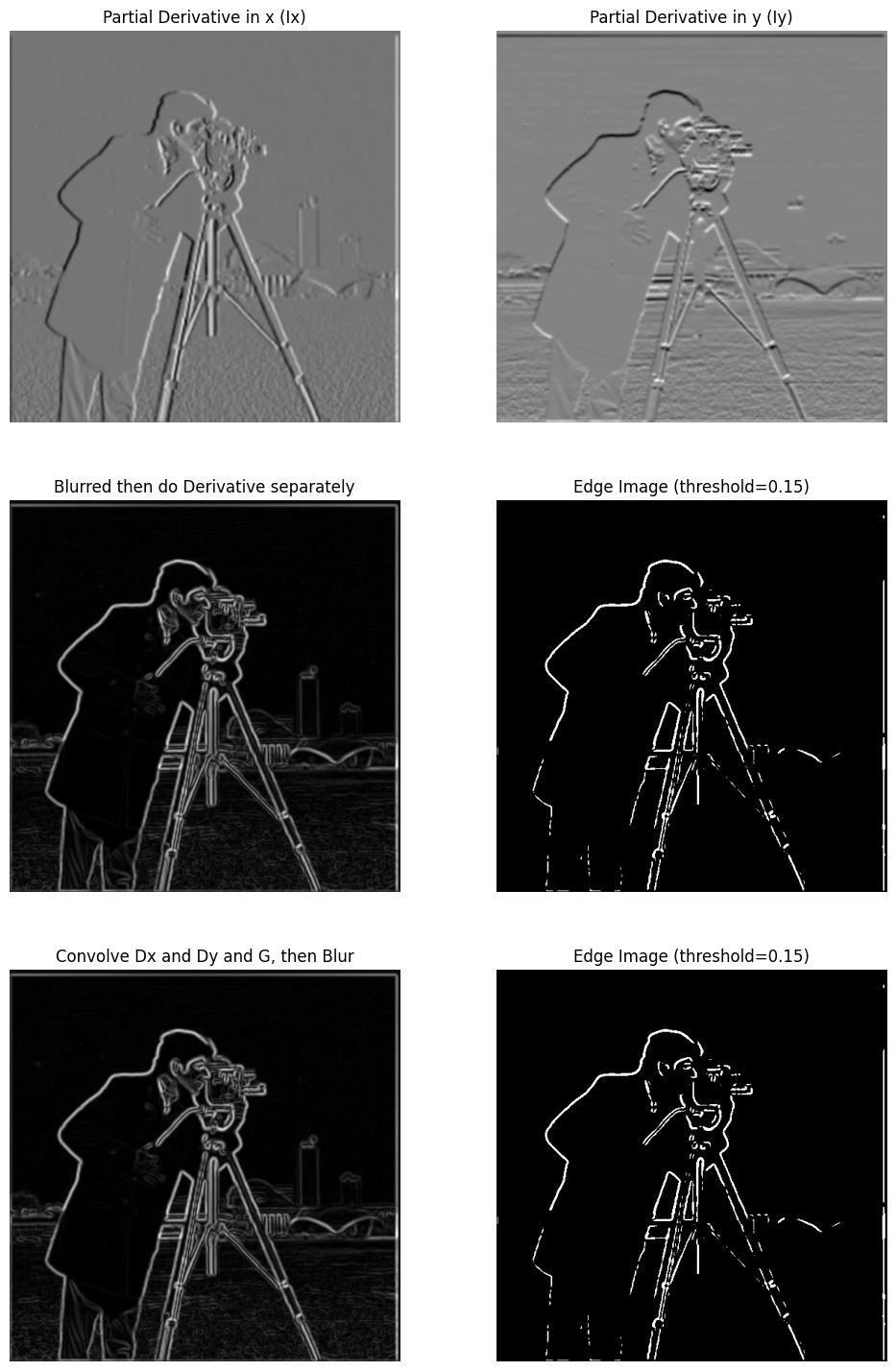
As we can see from the results, both methods can help remove the noise. These methods leave a clear edge for the image.

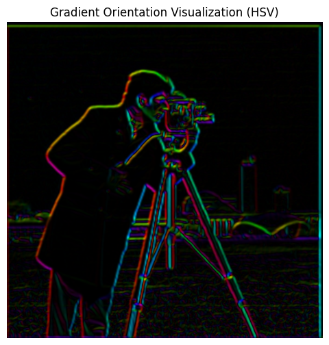
Bells & Whistles

Part 2: Fun with Frequencies!

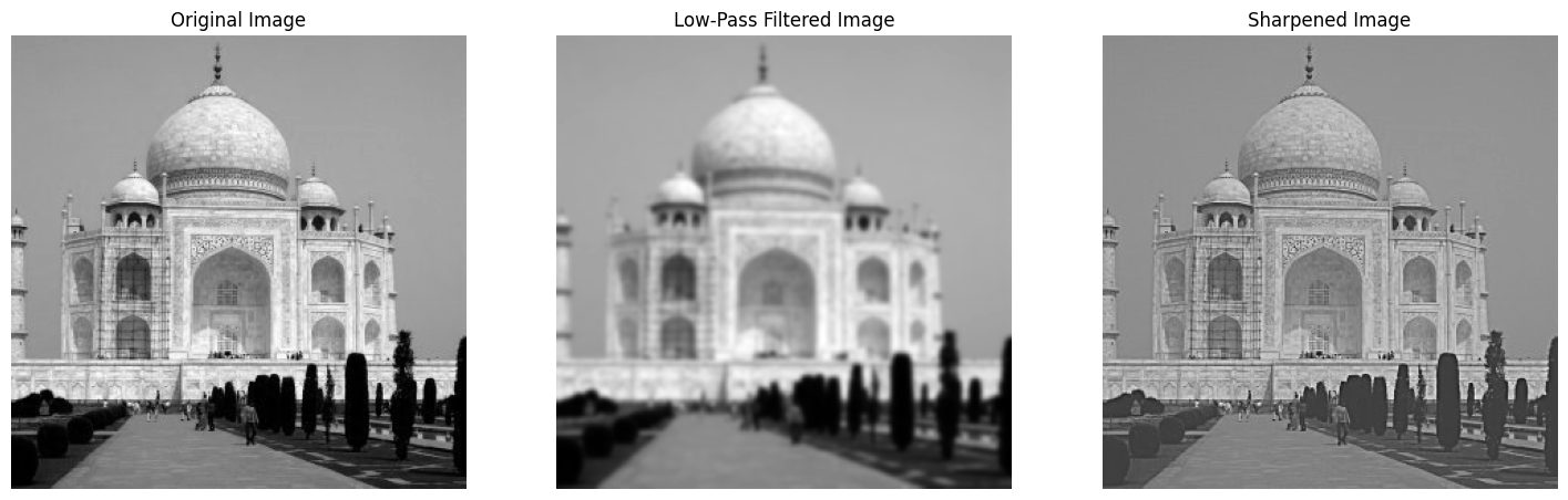
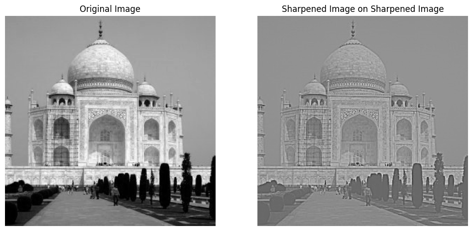
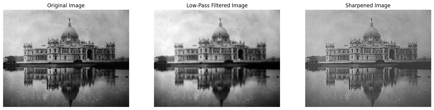
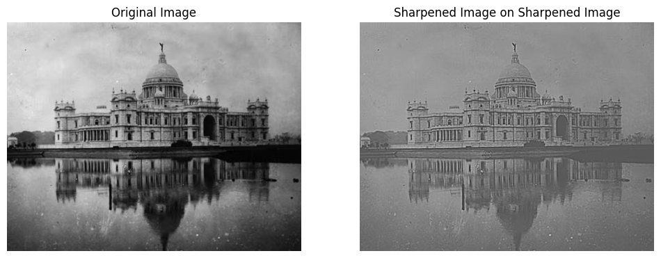
2.1 Image Sharpening

The image sharpening is rather simple after all the work we have done. We can simply use the gaussian kernel to get the low-pass filtered image and then subtract it from the original image to get the high-pass filtered image. Adding the high-pass filtered image to the original image will give us the sharpened image. The following are the results of using taj.jpg and kolkata.jpg.

2.2 Hybrid Images

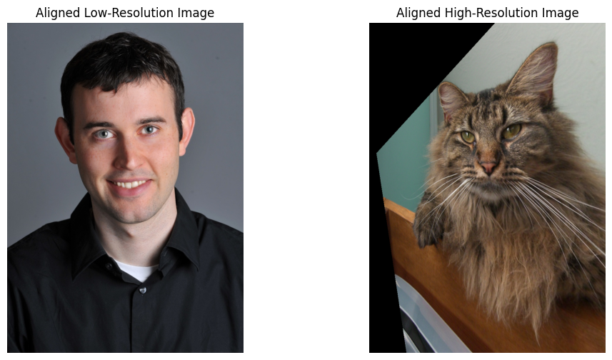
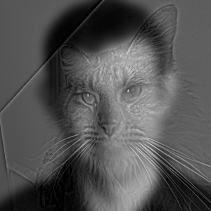
This is the most interesting part of the whole project, I get the change to implement some of the ideas I have been thinking about for a long time. Hybrid images are using two images with different frequencies to create a new image. And the first step is to align the two images.

I have tried to use the original code to align but I find that for the example shown (the man and the cat), I cannot get the result I like as the size of the face of the man and the cat are too different. Therefore, I implement another method using 4 dots to align the two images and conduct a transformation to align the two images. This way I can ensure that the size of the face of the man and the cat are the same. (Or at least better than the original alignment method.)

Then, the hybrid process is as follows:

Calculate the low-pass filtered image of the two images
Calculate the high-pass filtered image of the second image using the calculated low-pass filtered image
Add the high-pass filtered image of the second image to the original image to get the hybrid image

In this process, it is crucial to choose the right cutoff frequency used in the Gaussian filter. To remove the high-frequency components in the first image, we need to choose a higher cutoff frequency. For the second image, we need to choose a lower cutoff frequency to remove the low-frequency components and leave the high-frequency components.

The choice of the cutoff frequencies is really picture-based and to make the result look good, one has to choose the cutoff frequencies carefully.

Cutoff frequecies Sigma for the first image: 15, for the second image: 5

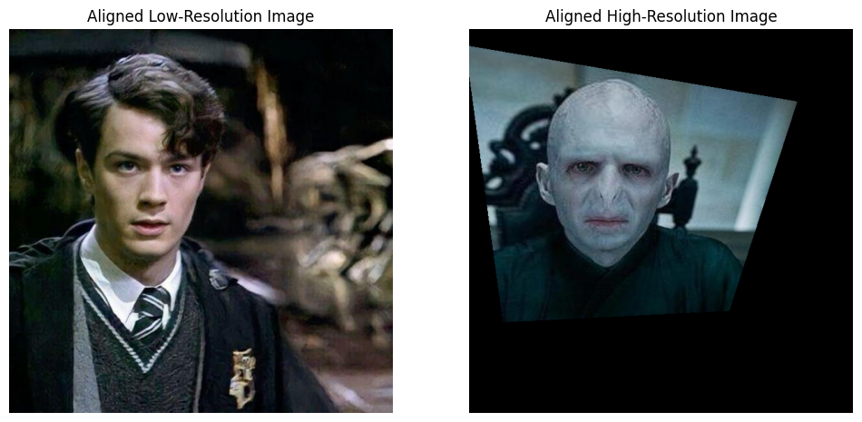
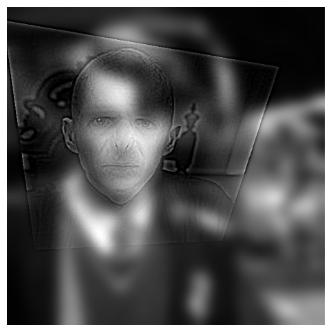
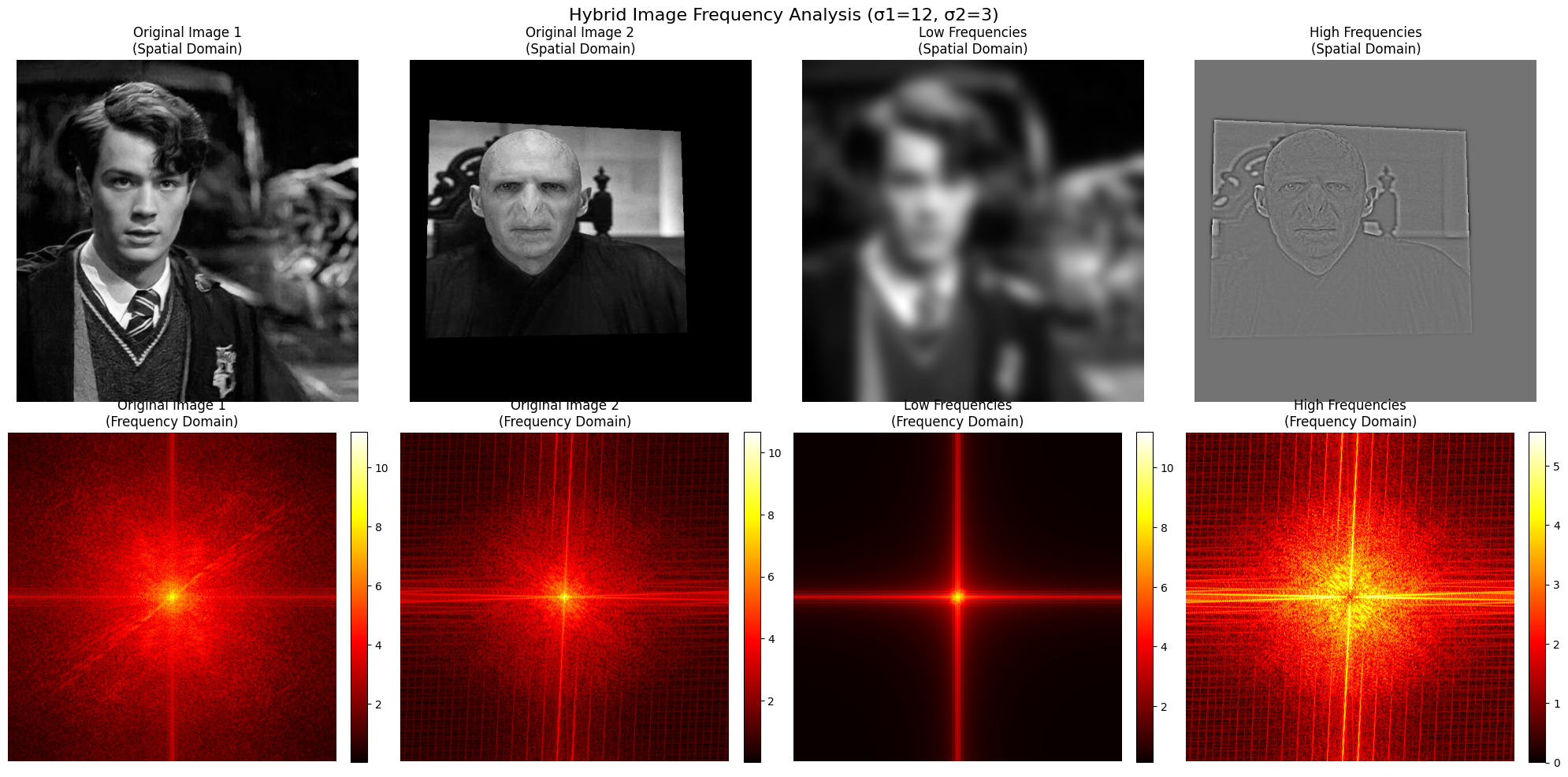
I am always a big fan of tv series and films that contain some kind of hidden characters or double identities with contrast, I think it will be a good time to implement this using hybrid image as you can see different people from near and far. This is a hybrid image of young Tom Riddle and Lord Voldemort.

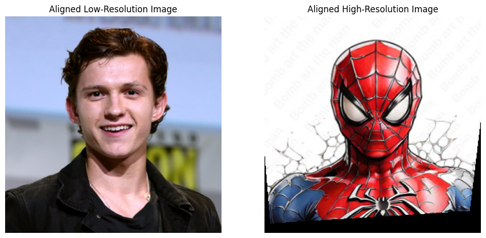
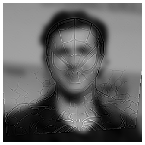
And here is a hybrid image of the spiderman and Tom Holland.

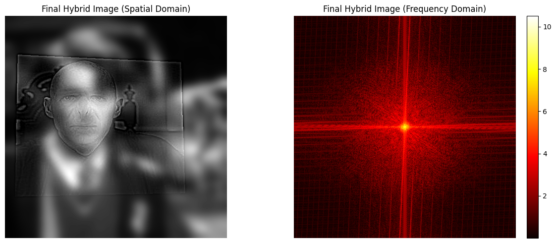
To showcase the whole process of hybrid image, I use the Voldemort picture to show how the frequency domain is like.

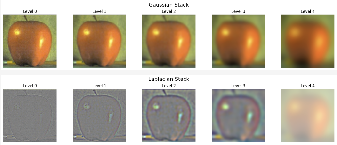
2.3 Gaussian and Laplacian Stacks

In this part, I try to implement the Gaussian and Laplacian stacks because it does not require upsampling and downsampling and it will be easier to calculate the original image from the Laplacian stacks using the stacks.

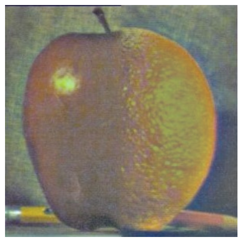
This is the result of the Gaussian and Laplacian stacks for the apple image.

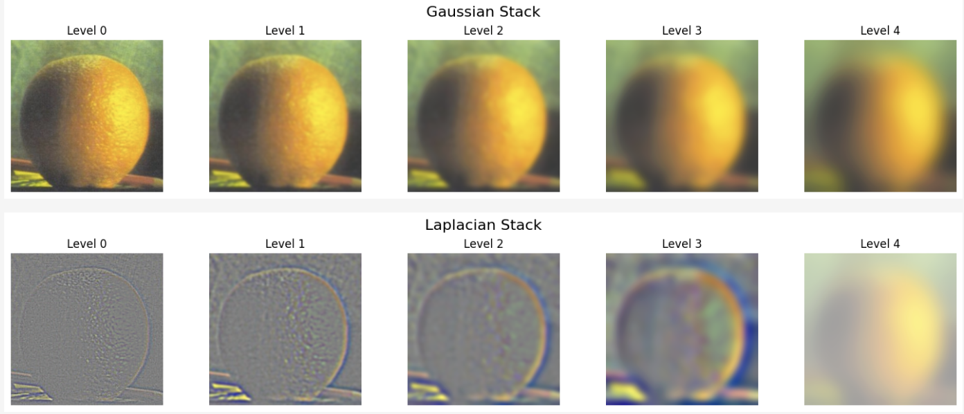
This is the result of the Gaussian and Laplacian stacks for the orange image.

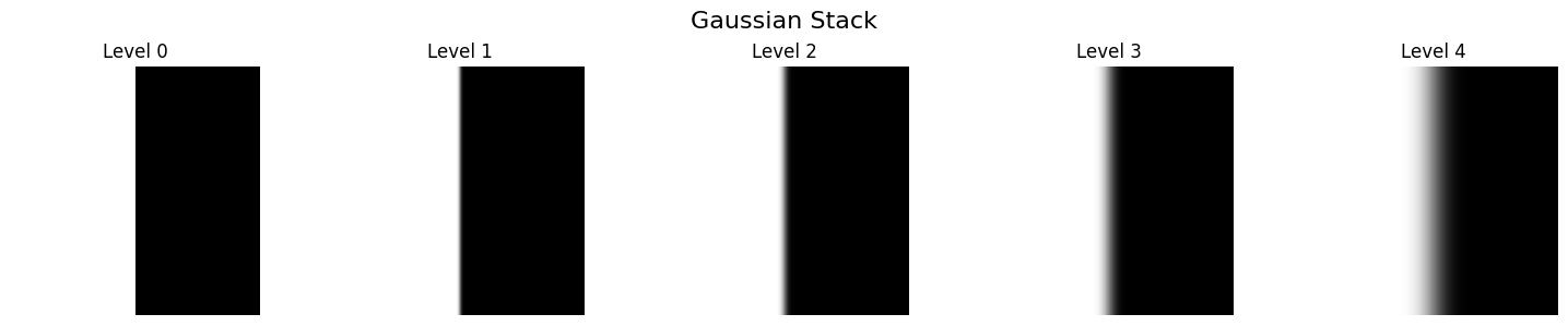
This is the result of the Gaussian stacks for the mask image.

And here is where I use the images from the Gaussian and Laplacian stacks to form the ‘oraple’ image.

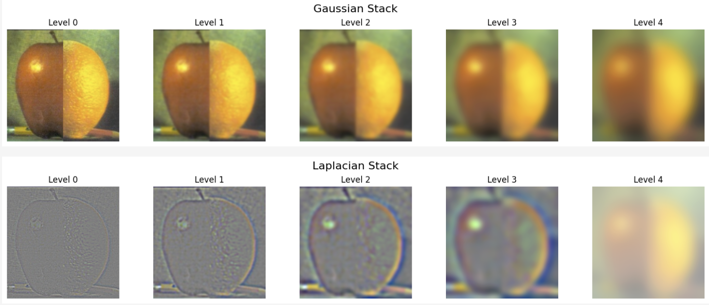
2.4 Multiresolution Blending

The blending process can be viewed as a multi-resolution blending process. Here are the main steps I take:

Prepare two images and a mask. (These should be of the same size.)
Compute the Gaussian and Laplacian stacks for two images. Compute the mask gaussian stacks.
Blend the Laplacian stacks using: $L_{\text{hybrid}}[i] = L_{\text{picture 1}}[i] * mask[i] + L_{\text{picture 2}}[i] * (1 - mask[i])$
Blend the lowest level of the Gaussian stacks using: $G_{\text{hybrid}}[0] = G_{\text{picture 1}}[0] * mask[0] + G_{\text{picture 2}}[0] * (1 - mask[0])$
Add up the lowest level of the Gaussian stacks and all levels of the Laplacian stacks to get the final image.

The result is quite good!

I have to note that showing the result requires normalization as the laplacian results have negative values. So the color in the Laplacian results are not the same as in the gaussian results.

Apple and Orange Multiresolution Blending Result

And too I try to use the blending machenism to bridge the reality and the anime I like:

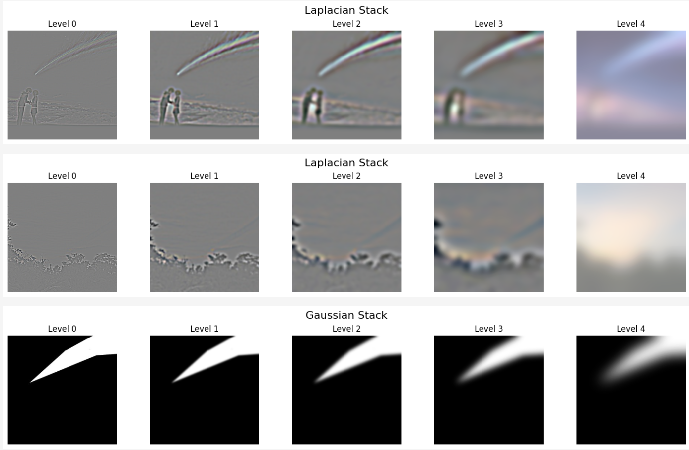
And here is the result of the blending:

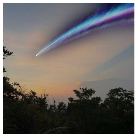
Reality and Anime: Your Name Multiresolution Blending Result

Here is another blending result using the main character inside the anime Your Name. (In this anime, Takiku and Mizuhan are the main characters and they go through a magic process of exchange their bodies.)

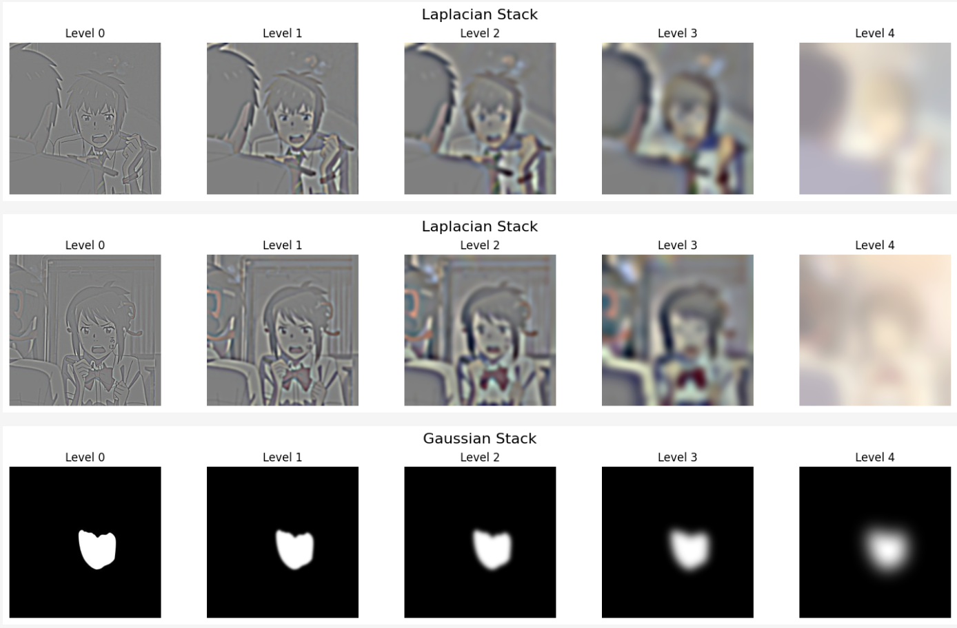
And here is the result of the blending:

Mizuhan and Takiku Blending Result

Conclusion

After learning all the techniques in Computer Vision, you can actually do some cool stuff with them! Including realize some of the ideas you have been thinking about for a long time! Merging reality and anime, transcending time and space, these are the power of Computer Vision!