[COMPSCI 180] Image Warping and Mosaicing

Overview

Here we only demonstrate the first part of the project 3, which aims to implement the image warping and mosaicing process.

Part A.1: Shoot the Pictures!

To get a perfect picture for the project, I take several tries and summarize some of the rules that we should follow:

1. Try not to move the camera, just try to rotate the camera.
2. Do not take pictures from far away, or the pictures are already at the same plane and the projection effect is not obvious.
3. Try to have more than 30% of overlap between the pictures, or after the projection, your warped image will experience severe distortion.
4. Do not use focal length that captures a wide field of view, this makes the image distorted badly.

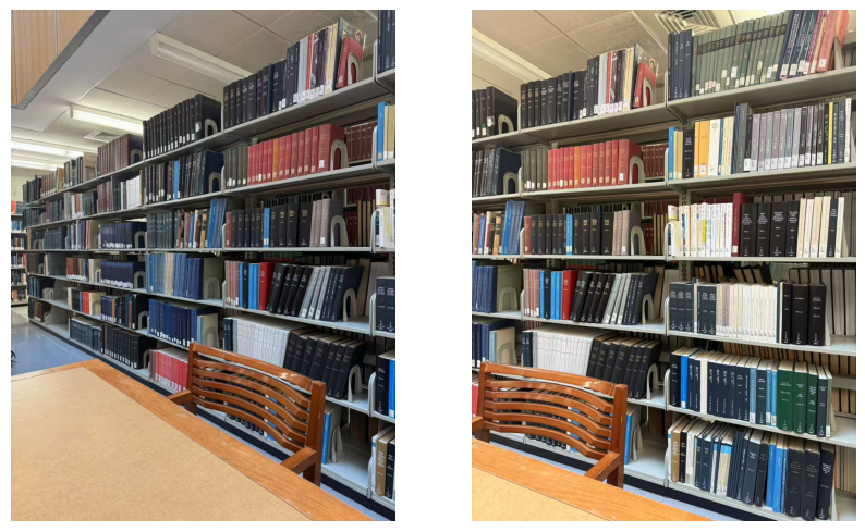
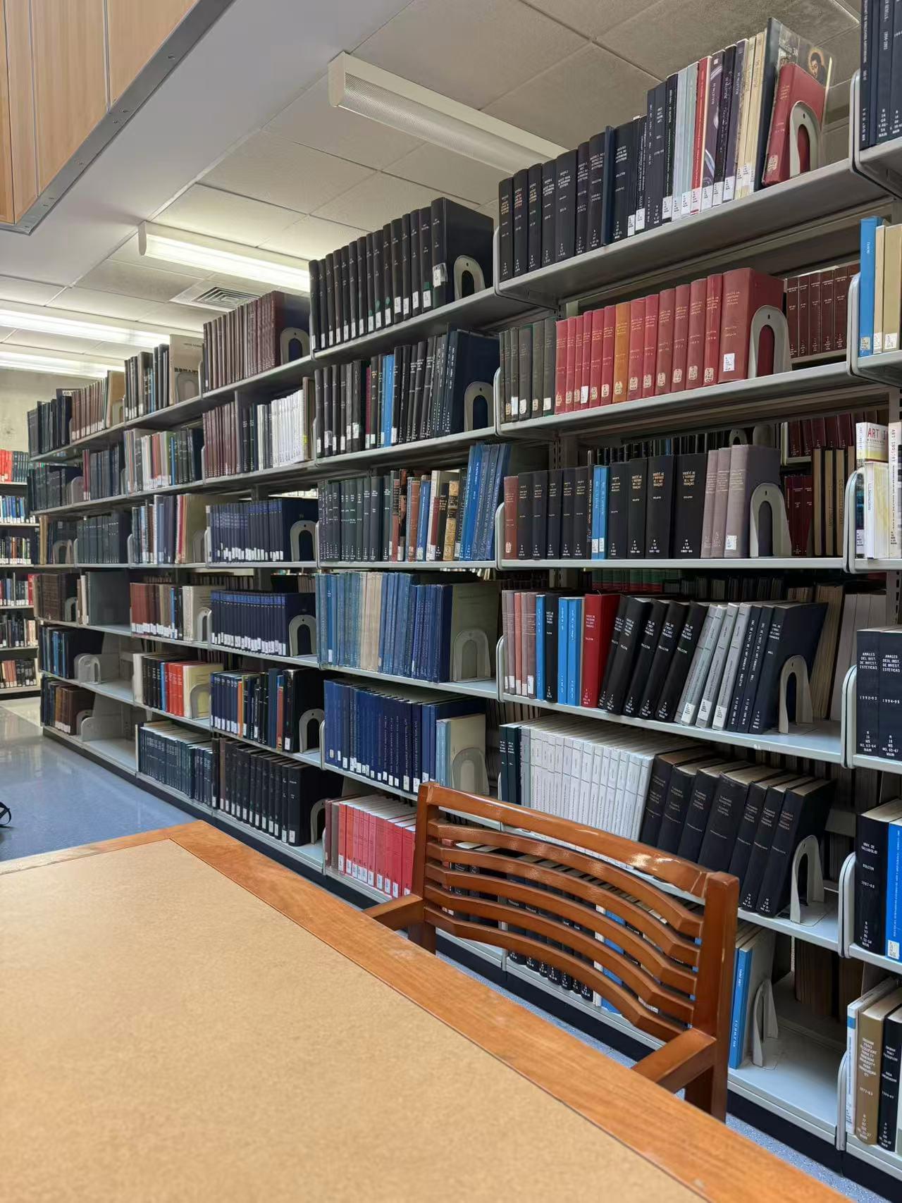
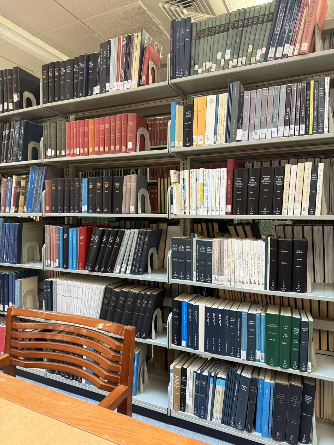
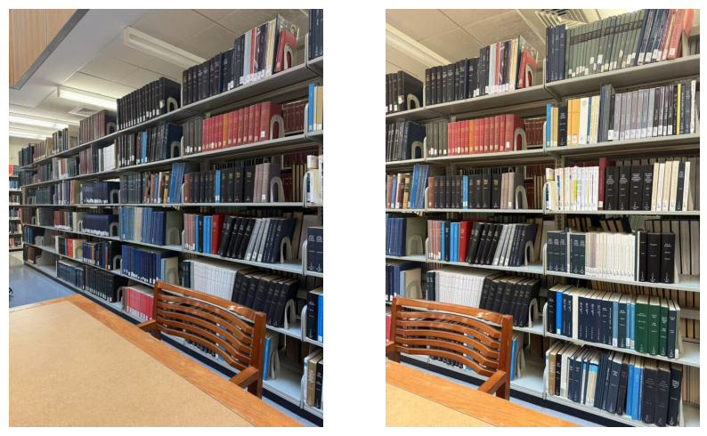
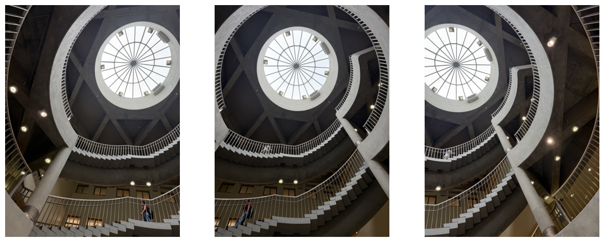
After several takes, the pictures took in the main stack library quite fit the requirements. Here is the demonstration:

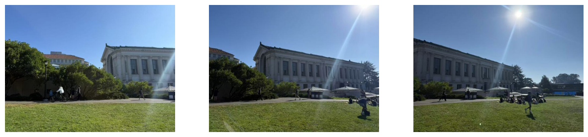
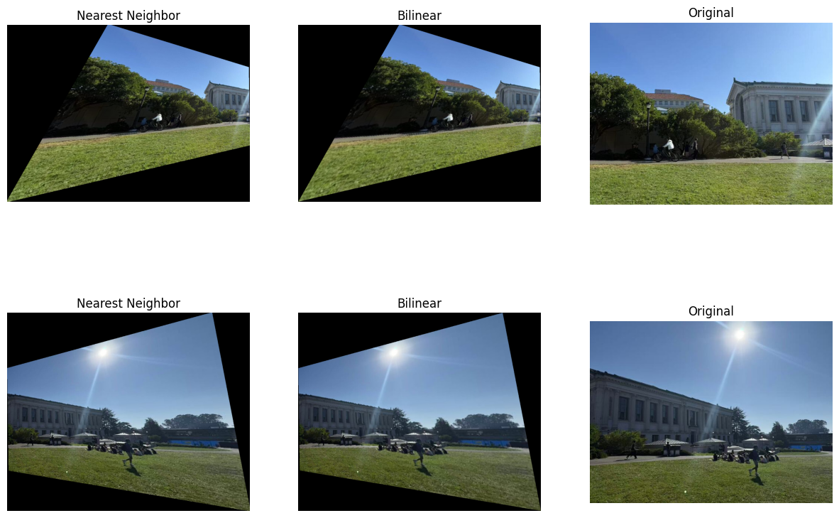
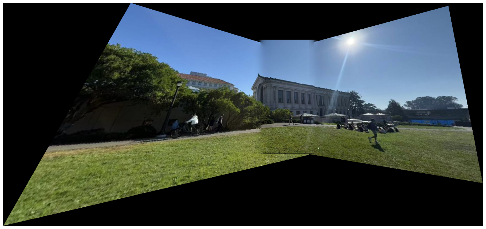
Also here is another example that I took for the Doe library:

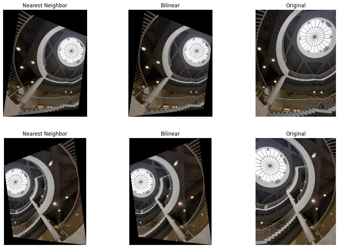
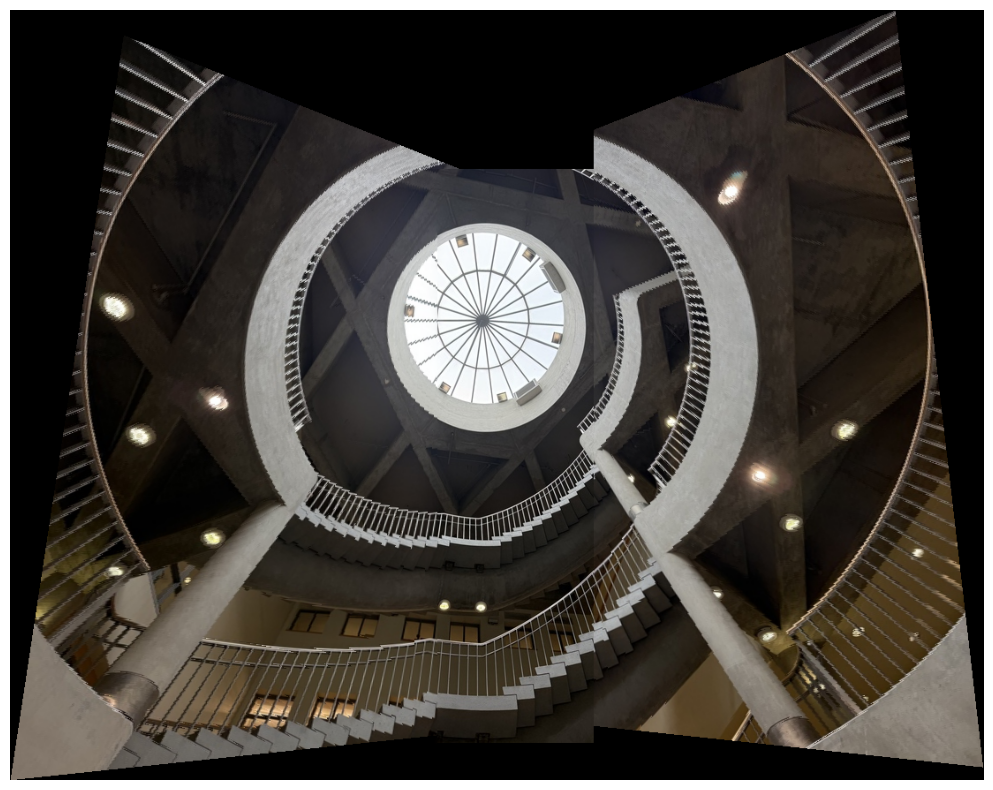
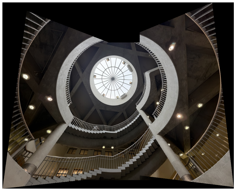
I really like the dome structure in the Main Stack Library so I also choose it to make the mosaic.

Part A.2: Recover Homographies!

Here we should implement the function H = computeH(im1_pts,im2_pts) to compute the homography matrix by using the coordinates of the points in both images.

First we have the transformation matrix $H$ that functions as belows:

$\lambda \cdot \begin{bmatrix} u \\ v \\ 1 \end{bmatrix} = H \begin{bmatrix} x \\ y \\ 1 \end{bmatrix} = \begin{bmatrix} h_1 & h_2 & h_3 \\ h_4 & h_5 & h_6 \\ h_7 & h_8 & h_9 \end{bmatrix} \begin{bmatrix} x \\ y \\ 1 \end{bmatrix}$

For one point, we can transform the above equation to a matrix equation:

$\begin{aligned} \lambda \cdot u_i &= h_1 \cdot x_i + h_2 \cdot y_i + h_3 \\ \lambda \cdot v_i &= h_4 \cdot x_i + h_5 \cdot y_i + h_6 \\ \lambda &= h_7 \cdot x_i + h_8 \cdot y_i + h_9 \\ \end{aligned}$

Then we can get the $A$ matrix with regards to one point:

$A = \begin{bmatrix} x_i & y_i & 1 & 0 & 0 & 0 & -x_i \cdot u_i & -y_i \cdot u_i \\ 0 & 0 & 0 & x_i & y_i & 1 & -x_i \cdot v_i & -y_i \cdot v_i \end{bmatrix} \begin{bmatrix} h_1 \\ h_2 \\ ... \\ h_8 \end{bmatrix} = \begin{bmatrix} u_1 \\ v_1 \\ ... \\ u_i \\ v_i \end{bmatrix}$

We need at least 4 points to solve for the 9 parameters in $H$ because there are in total 8 degrees of freedom. Write in batch form and we can get:

$\begin{bmatrix} a_1^T \\ a_2^T \\ ... \\ a_n^T \end{bmatrix} \begin{bmatrix} h_1 \\ h_2 \\ ... \\ h_8 \end{bmatrix} = \begin{bmatrix} u_1 \\ v_1 \\ ... \\ u_i \\ v_i \end{bmatrix}$

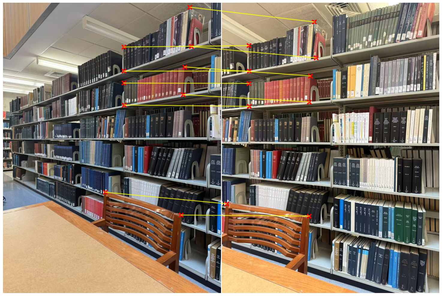
The corresponding points are get from the previous student’s work here. Thanks to this brilliant work!

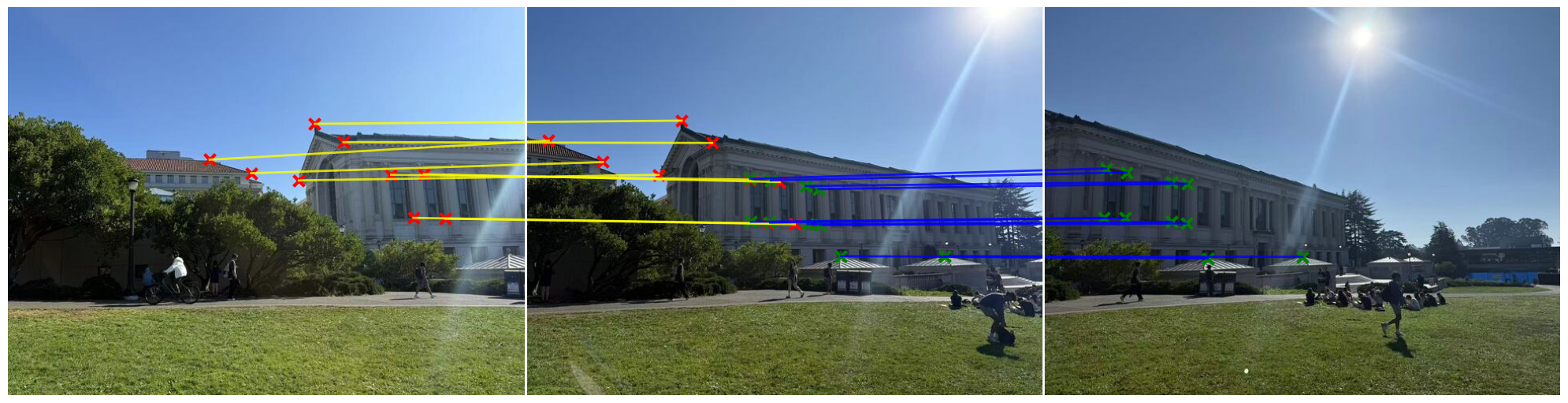
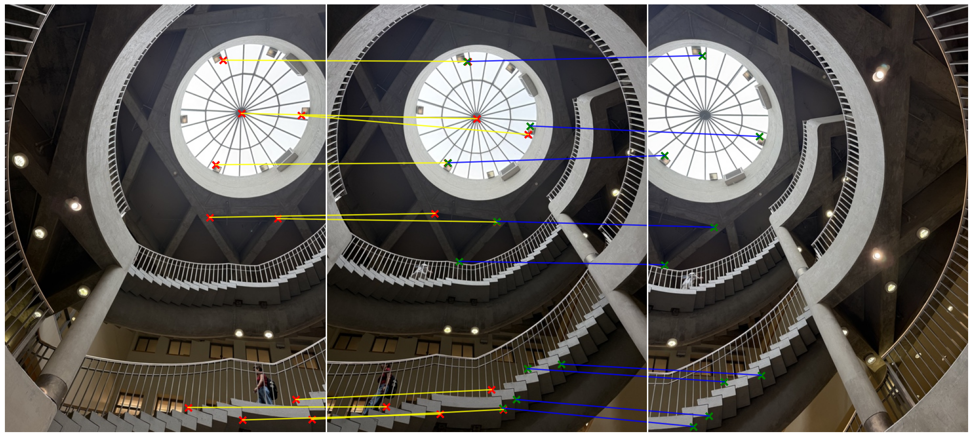
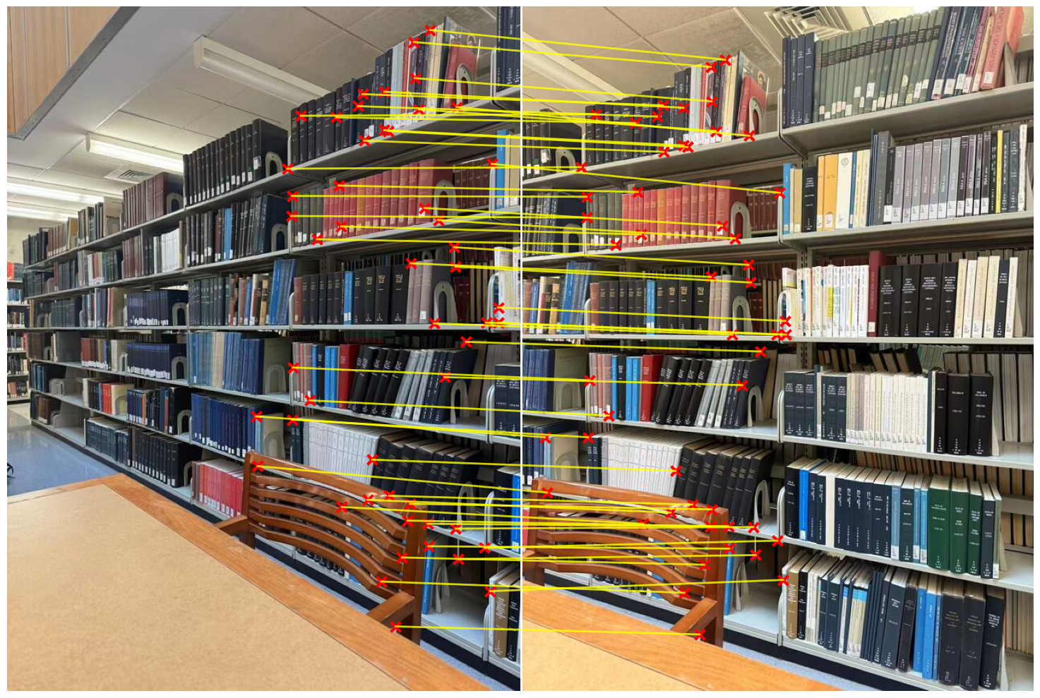
Let’s have a look at the matching points:

Part A.3: Warp the Images!

From the above part, we can see that we are getting a good homography matrix, however the images have black vacancies in between because we did not implement the interpolation. In this part, we need to warp the images to align them:

imwarped_nn = warpImageNearestNeighbor(im,H)
imwarped_bil = warpImageBilinear(im,H)

Implementing the warping functions we need to be aware of the following things:

1. We are trying to warp the image to the destination image, so we are mapping the coordinates at the exact location of the destination image, but because we are actually taking pictures with the same CoP but differen angle, we have to make a translation afterwards.

2. To decide on the translation, we need to find the minimum and maximum x and y coordinates of the warped image, and then subtract the minimum from the maximum to get the size of the translated image.

3. Then, to calculate the interpolated pixel values, we need to use the inverse of the homography matrix to map the coordinates back to the source image.

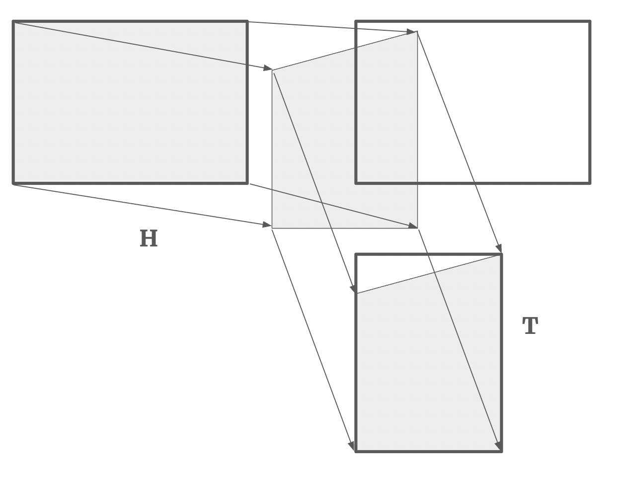
Here is the illustration of the translation process, we actually need to matrices, one for the homography transformation $H$ and one for the translation $T$.

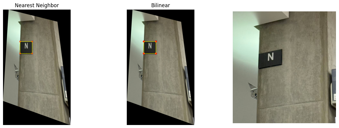
We first use the rectification process to ensure that our algorithm is actually working. Take a photo that contains a rectangular like in the figure having the N sign. Then we use the matching points as: [[160 260], [300 260], [160 400], [300 400]]. This indicates that we hope to transform the N sign to a square.

After testing out the result, I use both functions on the main stack library images and the Doe library images. Here is the result:

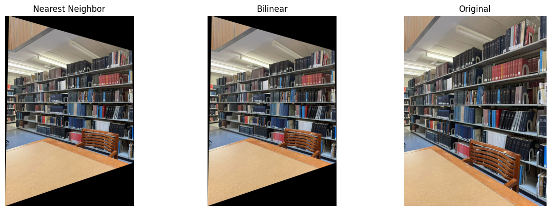
Image	Nearest Neighbor	Bilinear	Point Number
Main Stack Library	18.39 seconds	30.15 seconds	10
Doe Library Left	4.46 seconds	6.94 seconds	9
Doe Library Right	2.94 seconds	4.62 seconds	10
Dome Library Left	2.42 seconds	3.99 seconds	10
Dome Library Right	2.42 seconds	3.91 seconds	9

The time taken for both method is shown in the table above. We can see that the nearest neighbor method is usually faster than the bilinear method. As for the image quality, we can see in general both methods can produce a good result. However, if we zoom in on the upper left corner, we can see that using bilinear method can produce a smoother result. (There are these zigzag patterns in the line of the nearest neighbor method.)

Part A.4: Blend the Images into a Mosaic

For this part, we need to be careful about the size of the images because of the stretch and all the black vacancies. Also, we need to make sure that the mask is working properly. Here is an illustration of blending:

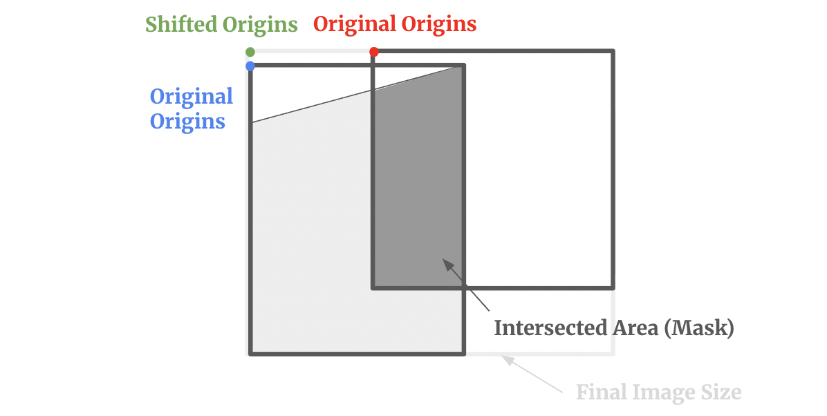
There is one thing that I need to stress that the size of the two original images might not have the same size.

1. We need to find the warped image coordinates in the system of the reference image.
2. Then we need to find the coordinates in the system of the reference image in the final image.

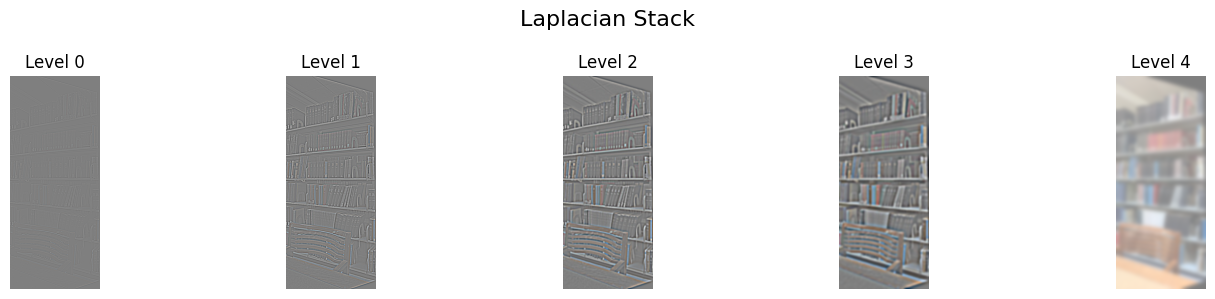
Here in this part, I use the Laplacian blending to blend the images together. However, usually the transformed images are big in size, therefore calculating the whole images will be very time-consuming. I try to calculate the overlap part of the original images and the warped images and then only blend the overlap part. This helps accelerate the process.

Therefore the whole 2-image blending process can be summarized as:

1. Warp & Align

   • Warp image_homo to align with image_ref using homography H
   • Calculate alignment info: shifts, final canvas size, and overlap mask region

2. Extract Overlap Region

   • Extract the overlapping pixels from both the warped image and reference image
   • Create a binary blend mask (left half = 1, right half = 0)

3. Build Pyramids

   • Create Laplacian stacks for each RGB channel of both overlap regions (multi-resolution frequency decomposition)
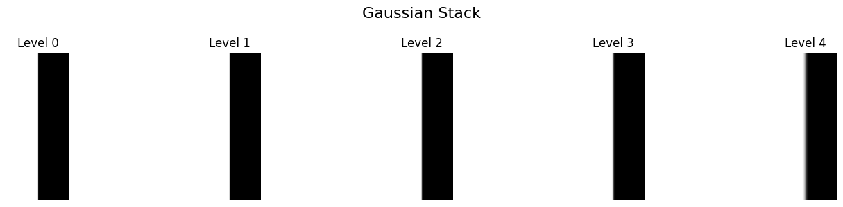
   • Create Gaussian stack of the blend mask (smooth transition weights)

4. Stack RGB Channels

   • Combine R, G, B Laplacian stacks into color pyramids

5. Blend at Each Pyramid Level

   • At each frequency level: $blended = warped \times mask + reference \times (1 - mask)$
   • This blends high frequencies sharply and low frequencies smoothly

6. Reconstruct Final Blend

   • Collapse the blended pyramid: start from coarsest level, add each finer level
   • Normalize the result

7. Compose Final Panorama

   • For each pixel in the final canvas:
     • If in overlap region: use blended result (seamless transition)
     • Else if in reference image: use reference directly
     • Else if in warped image: use warped directly

Here is the Laplacian stack of the warped images:

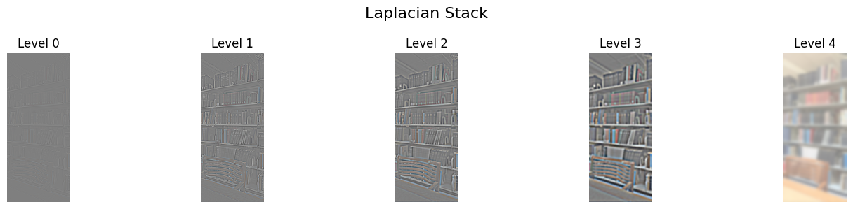
And here is the Laplacian stack of the original images:

The gaussian stack for the mask:

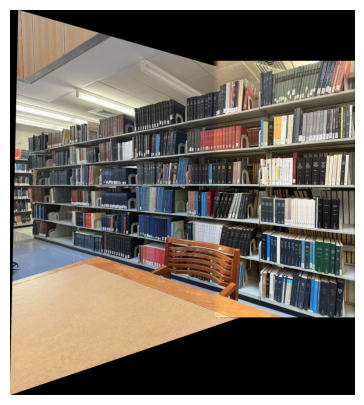
And here is the result of the blending for the main stack library:

The blending process for three images is basically the same as the two images. We need to warp the left and the right images to the middle image and then blend them together. Here is the result for the Doe library:

Here is the result for the dome of the Main Stack Library:

Although there are still this inconsistencies on the color and the size, the results are still quite good.

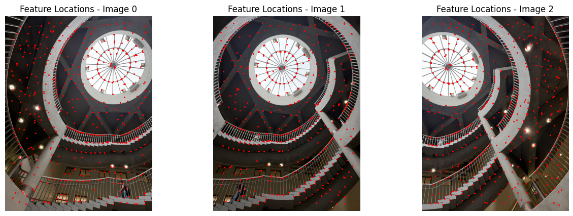
Part B.1: Harris Corner Detection

Here we are trying to first use Harris Corner Detection to detect the corners of the image and then use Adaptive Non-Maximal Suppression (ANMS)to select some of the interest points. The logic of using ANMS is that interest points are suppressed based on the corner strength $f_{HM}$ , and only those that are a maximum in a neighbourhood of radius $r$ pixels are retained. Therefore the algorithm is as follows:

$r_i = \min_{j} |x_i - x_j|, \text{s.t. } f(x_i) < c_{robust} f(x_j), x_j \in I$

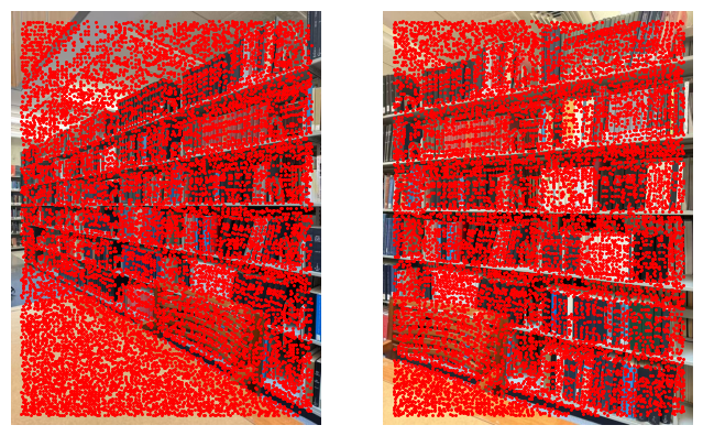
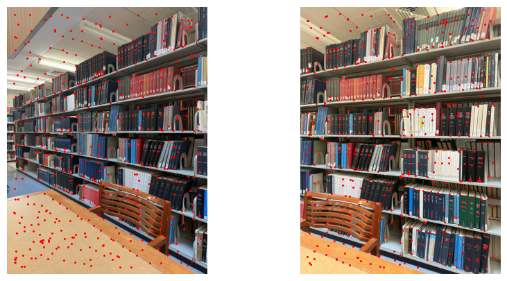
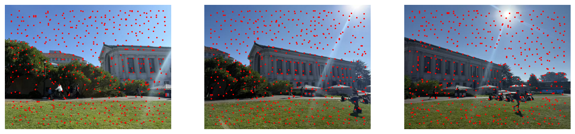
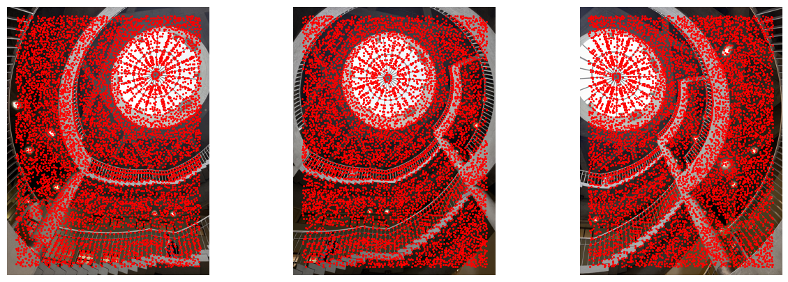
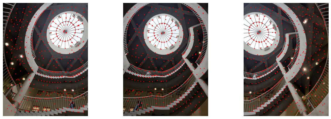
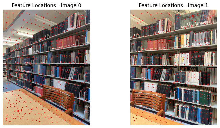
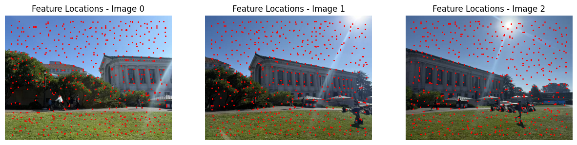
Here is the original image, the corner detection result and the ANMS result (by selecting the top 500 points):

Original Image

→

Harris Corner Detection

→

ANMS Result (Top 500)

DOE - Original Image

→

DOE - Harris Corner Detection

→

DOE - ANMS Result (Top 500)

DOME - Original Image

→

DOME - Harris Corner Detection

→

DOME - ANMS Result (Top 500)

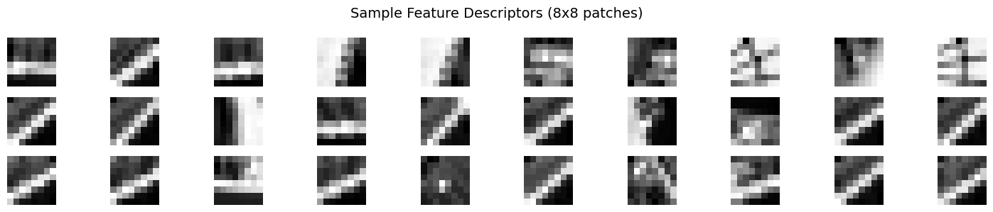
Part B.2: Feature Descriptor Extraction

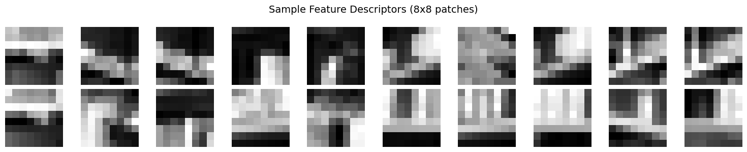
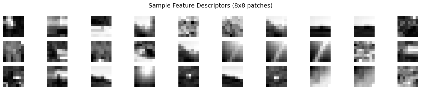
Here we use a simple descriptor extraction algorithm that creates local feature descriptors for each detected interest point. For each feature point, a square window of a specified size (window_size, e.g., 40x40 pixels) centered at that point is extracted from the grayscale image. This window is then resized to a smaller, fixed patch size (e.g., 8x8 pixels) to achieve a compact representation. Before storing the descriptor, the patch is normalized by subtracting its mean and dividing by its standard deviation to ensure invariance to linear changes in brightness and contrast. The resulting descriptors are suitable for matching, as they encode normalized local structure around each interest point in a consistent, compact vector.

Steps:

1. For each given coordinate (interest point), extract a square window from the input image centered at that coordinate.
2. If the window goes out of image bounds, skip that point.
3. Resize the window to a smaller, fixed resolution (e.g., 8x8) using anti-aliasing for smoothness.
4. Normalize the patch to have zero mean and unit variance.
5. Store all normalized patches as feature descriptors for further matching tasks.

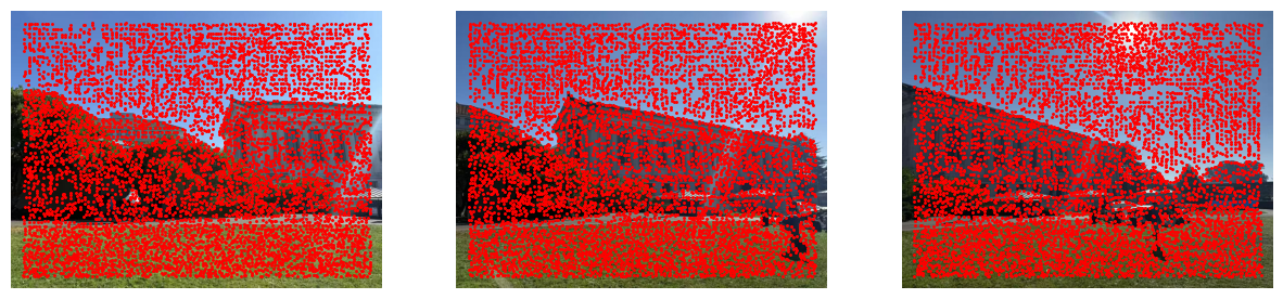
The result of the descriptor extraction is shown below:

Part B.3: Feature Matching

The feature matching algorithm proceeds in the following stages:

1. Distance Calculation: For each feature descriptor in the first image, we compute the pairwise distance (usually L2 norm) to every descriptor in the second image. This results in a distance matrix where each entry represents the difference between a pair of descriptors from the two images.

2. Nearest Neighbor Matching: We then match each feature based on this distance matrix. Using the “ratio test” (inspired by Lowe’s SIFT matching), the smallest and second-smallest distances for each descriptor are identified. If the ratio of the smallest to the second-smallest is below a given threshold (Here we choose 0.6 based on the essay), the match is considered reliable and kept. This helps filter matches that are ambiguous or likely to be incorrect.

This approach ensures feature matches are both distinctive and robust, allowing for reliable correspondence between interest points across different images.

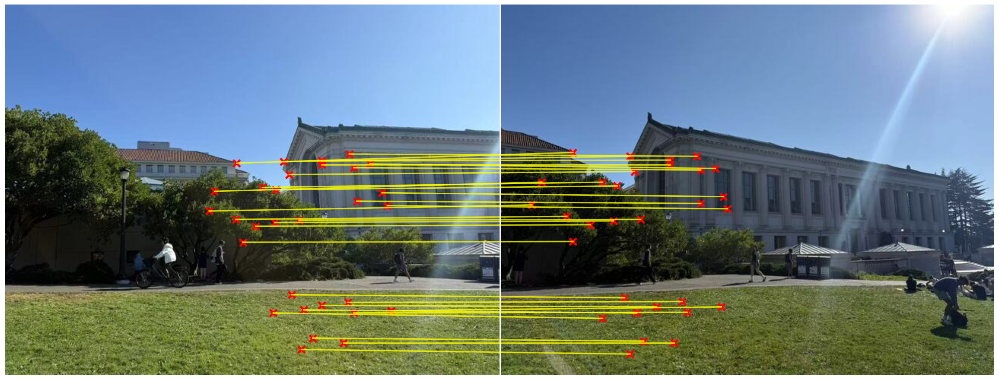
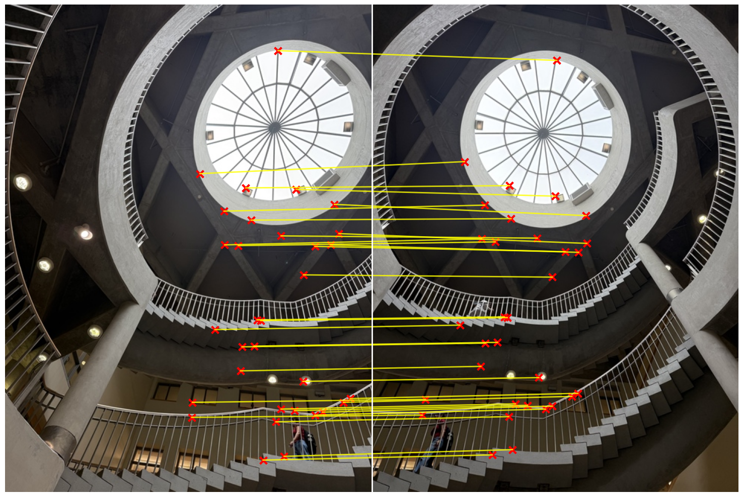
The result of the feature matching is shown below:

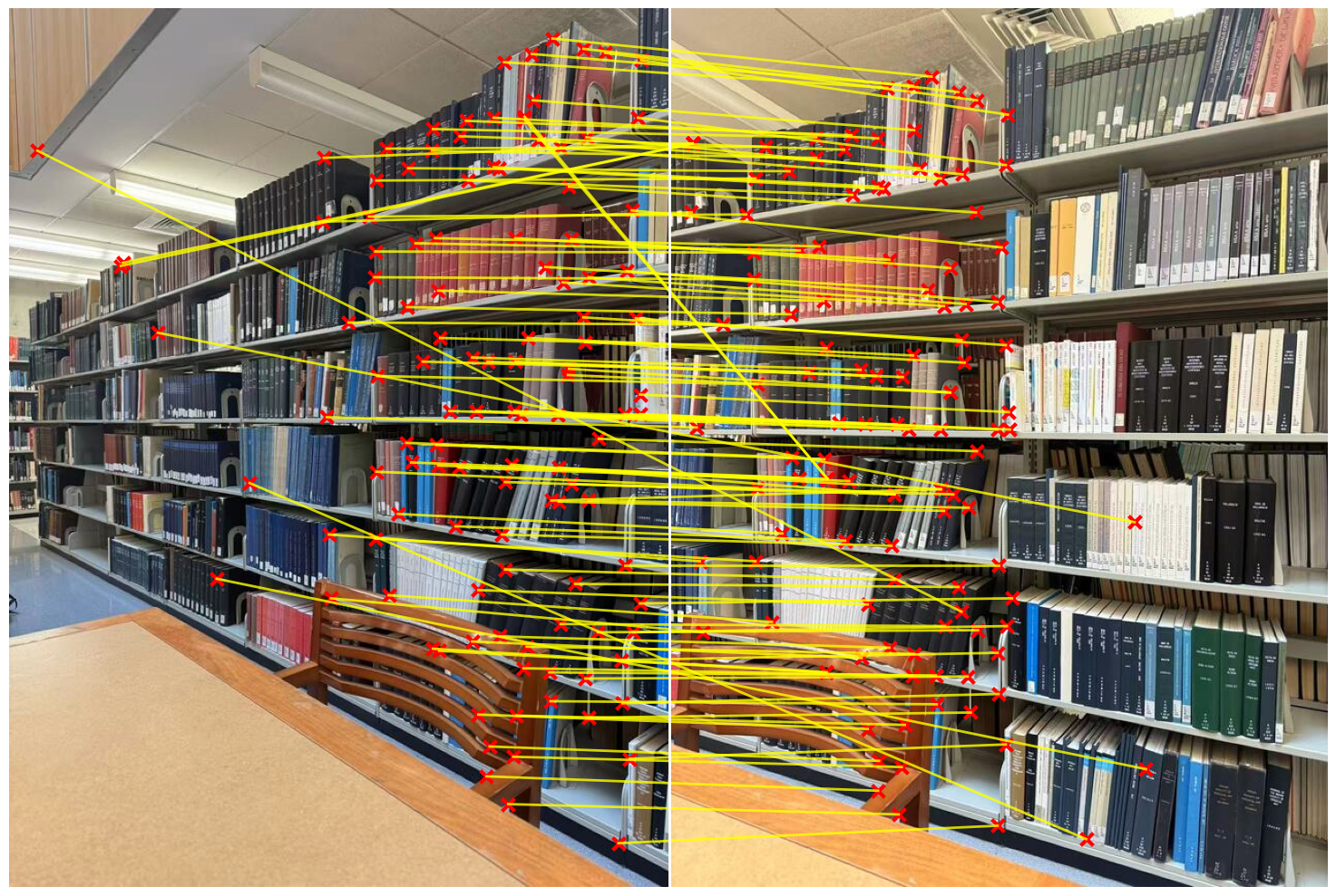
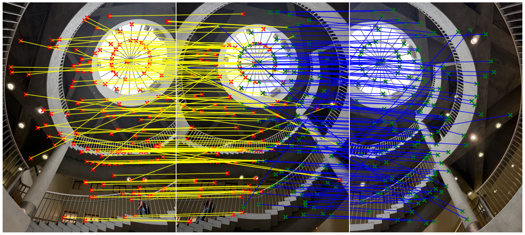
We can see that there are still a lot of bad matches, therefore we need to use the RANSAC to filter out the bad matches.

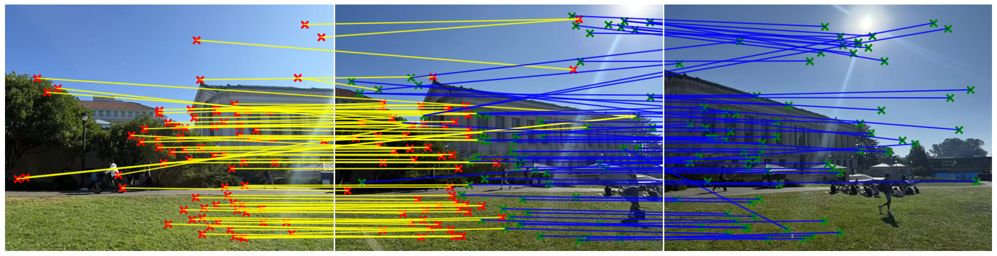
Part B.4: RANSAC

The RANSAC algorithm is used to estimate the homography matrix. The algorithm is as follows:

1. Randomly select 4 matches from the feature matching result.
2. Estimate the homography matrix using the 4 matches.
3. Calculate the inlier matches using the homography matrix.
4. Repeat the process for a certain number of iterations or until the number of inlier matches is greater than a certain threshold.
5. Return the coordinates of the inlier matches.
6. Calculate the homography matrix using the coordinates of the inlier matches.

We can first see that the RANSAC can help filter out the bad matches and get the correct matches out.

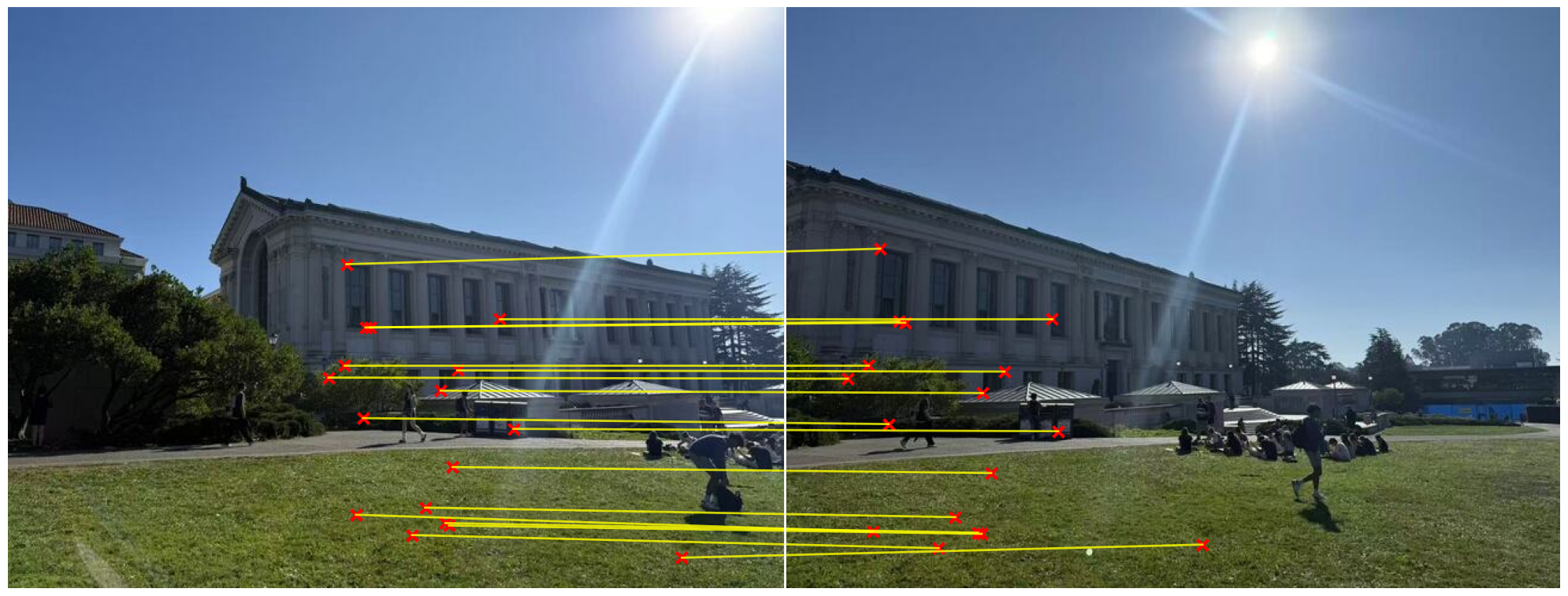
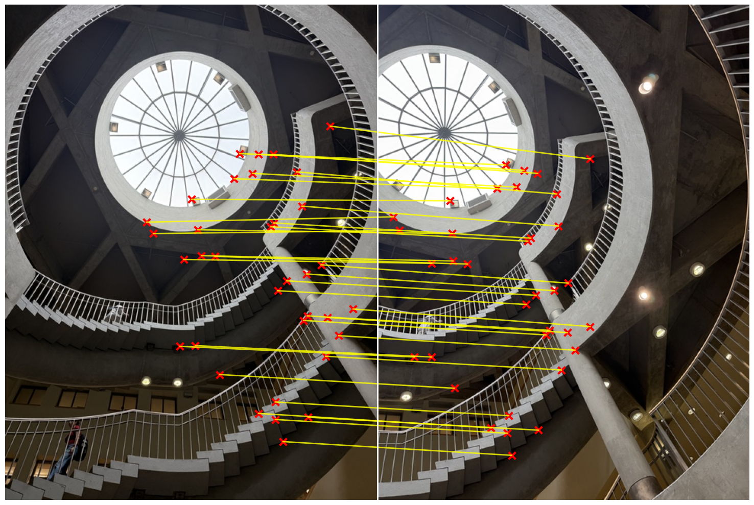
The stitching result is shown below:

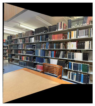
Library

Automatic

Artificial

← Drag the slider to compare

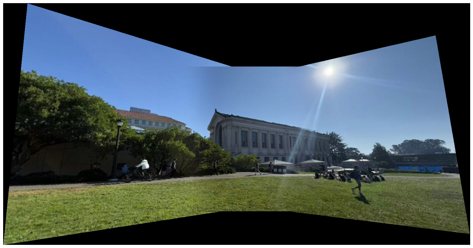
DOE

Automatic

Artificial

← Drag the slider to compare

DOME

Automatic

Artificial

← Drag the slider to compare

Library Manual Stitching Result

Library Automatic Stitching Result

Doe Manual Stitching Result

Doe Automatic Stitching Result

Dome Manual Stitching Result

Dome Automatic Stitching Result

The most prominent difference you can spot is in the doe stitching (You can see that in the automatic stitching the road is more consistent), because the features in the picture are not as distinct as the library and dome. Therefore by selecting the matches by hand will really result in a worse result. Therefore, here the automatic stitching is better.

Conclusion

After learning the image warping and mosaicing, I have a deeper understanding of the image processing and the computer vision. I also have a deeper understanding of the homography matrix and the RANSAC algorithm. This project is a great practice for me to apply the knowledge I have learned in the class to the real world problems. As we can see from the result, the automatic stitching is better than the manual stitching, especially for the doe library. I am surprised that even with the simplest detection and matching algorithm, we can still achieve relatively good results.