[COMPSCI 180] Neural Radiance Field!

Part 0: Calibrating Your Camera and Capture a 3D Scan!

Here is the 3D scan of my doggy! You can drag and scroll to explore different views.

Drag or scroll to explore different views

Part 1: Fit a Neural Field to a 2D Image

Part 1.1: Model Architecture

Property	Description
Model Type	Multi-Layer Perceptron (MLP) with sinusoidal positional encoding
Purpose	2D coordinate-based neural radiance field (NeRF-style) for image regression
Input	2D spatial coordinates (x, y)
Output	RGB color values (r, g, b) in range [0, 1]
Number of HiddenLayers	3
Layer Width	128
Sinusoidal Encoding	Sinusoidal encoding with L = 10 frequency bands
Activation Function	ReLU for hidden layers, Sigmoid for output
Optimizer	Adam
Learning Rate	1e-2
Loss Function	Mean Squared Error (MSE)

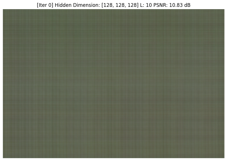
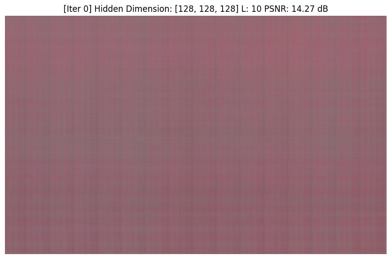
Part 1.2: Training progression visualization

Training Step (Standard Image): 0 Training Step (Self-Chosen Image): 0

Part 1.3: Grid for demonstrating the effect of hidden dimensions and L

Dimension/L (dB)	4	10	16	25
[128, 128, 128]	26.03	27.81	27.67	27.44
[256, 256, 256]	26.01	28.33	28.42	27.69

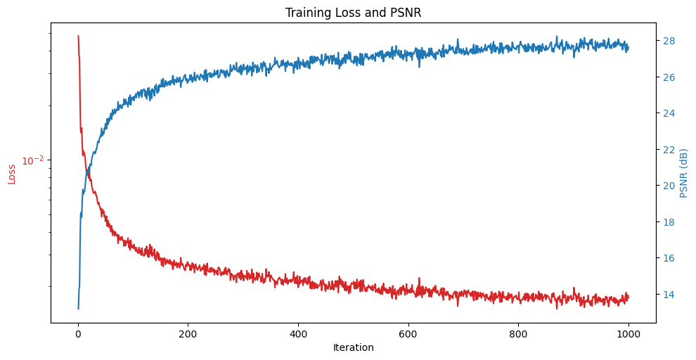
Part 1.4: PSNR Curve when training

This is the PSNR curve and Loss curve when training with the self-chosen image. The dimensions are [128, 128, 128] and L = 10.

Part 2: Fit a Neural Radiance Field from Multi-view Images

Now we move on to the more challenging part of implementing a Neural Radiance Field from multi-view images.

Part 2.1: Brief Introduction

The NeRF model part can be devided into the following steps:

1. We first need to calculate the rays from the cameras.
2. After we get the rays, we need to sample the points along the rays.
3. We need to implement the models, the models take the point coordinates and the camera rays as input and output the color and density of the point.
4. Then we need to integrate the density along the ray to get the final color of the ray.

Calculate rays from cameras

Follow the instruction given, I implement 3 functions for calculating the rays from cameras namly:

1. transfrom : This function transforms a point from the camera coordinates to world coordinates. (Extrinsic Transformation Matrix)
2. pixel_to_camera : This function transforms a pixel to the camera coordinates. (Intrinsic Transformation Matrix)
3. pixel_to_ray : This function transforms a pixel to the ray direction in the camera coordinates. It first us the pixel_to_camera to get the camera coordinates of the pixel, then use the camera coordinates to get the ray direction in the camera coordinates. ray_o represents the camera origin direction in the world coordinates and ray_d represents the ray direction in the world coordinates.

After the process, we can get the rays in the world coordinates. Then we can sample the points along the rays to get the color and density of the point.

Sample points along the ray

Here I just implement a class RaysData for handling all the arrays in a group of images. Inside the class, I implement the function sample_rays by first sampling num_images number of images from the image pool and then sample tot_samples/num_images number of rays for each image.

After sampling the rays, we need to sample along the rays by using the sample_along_rays function. This function is implemented by first sampling num_samples number of points along the ray and then transform the points to the world coordinates.

Implement the models

Here I implement a class NeRF3D inheriting from torch.nn.Module class. The class is used to implement the NeRF model.

Component	Input	Output	Description
Inputs	x ∈ ℝ³, ray_d ∈ ℝ³	—	3D point and ray direction
Position Encoding (x)	(B, 3)	(B, 63)	10-frequency sinusoidal encoding
Direction Encoding (ray_d)	(B, 3)	(B, 27)	4-frequency sinusoidal encoding
MLP Trunk	(B, 63)	(B, 256)	4-layer MLP with ReLU activations
Skip Block	(B, 256 + 63)	(B, 256)	Combines trunk output and encoded position
Density Head	(B, 256)	(B, 1)	Predicts volume density (Softplus)
Feature Layer	(B, 256)	(B, 256)	Latent feature for color prediction
Color Head	(B, 256 + 27)	(B, 3)	Predicts RGB color (Sigmoid)
Outputs	—	density ∈ ℝ¹, color ∈ ℝ³	Final NeRF outputs per sample

Integrate the density along the ray

Then after we put the 3D coordinates and rays into the model, we can get the density and the color of the point. Then we need to integrate the density along the ray to get the final color of the ray by implementing the volrend function.

In the function, we use the t_val from the sample_along_rays function to know that after the purtubation what is the distance between each sample point. Then we can use the density to integrate the color along the ray.

Training the model

Then we set the optimizer to be Adam and the loss function to be the mean squared error. We then train the model for 1000/5000/10000 steps based on the task we have.

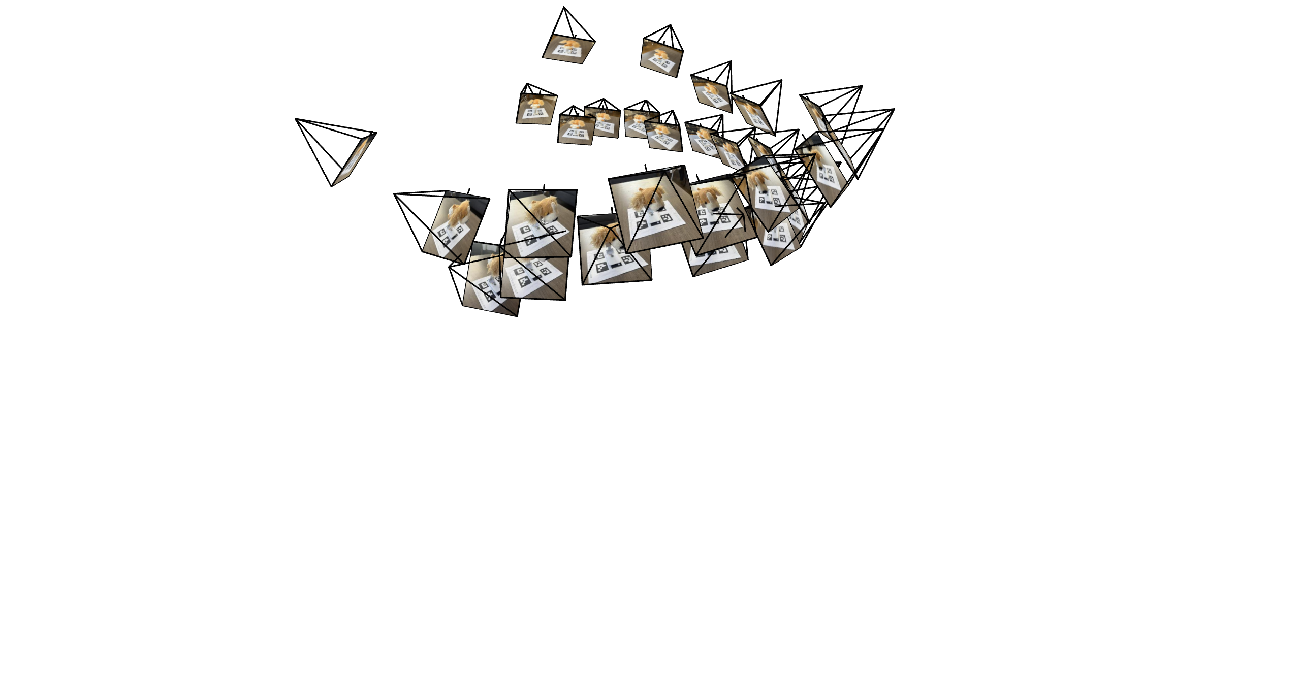
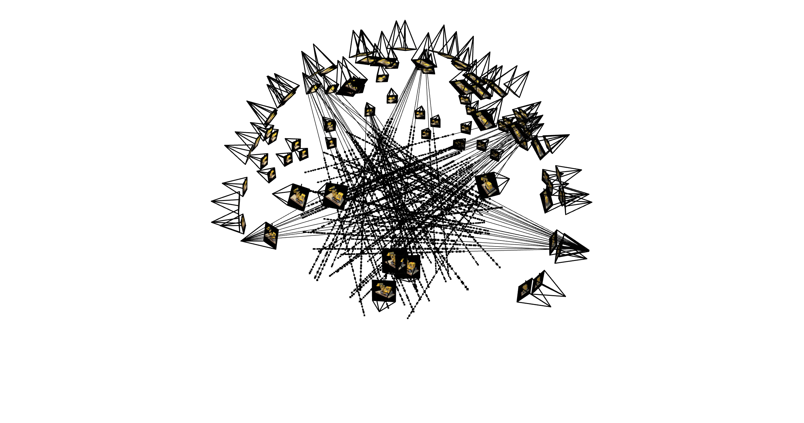
Part 2.2: Visualization of rays and samples with cameras

This is the visualization of rays and samples with cameras. We can see that the rays are sampled from the camera and the samples are sampled from the rays.

Drag or scroll to explore different views

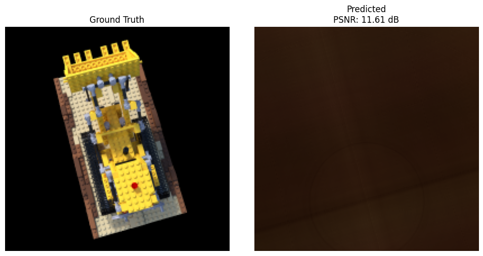
Part 2.3: Training visualization / PSNR curve

Training Step: 50 PSNR: 11.61 dB

Training Step: 50 PSNR: 24.1 dB

Part 2.4: Spherical rendering video

After training the model, we can render the test scenes in spherical coordinates.

Test Video

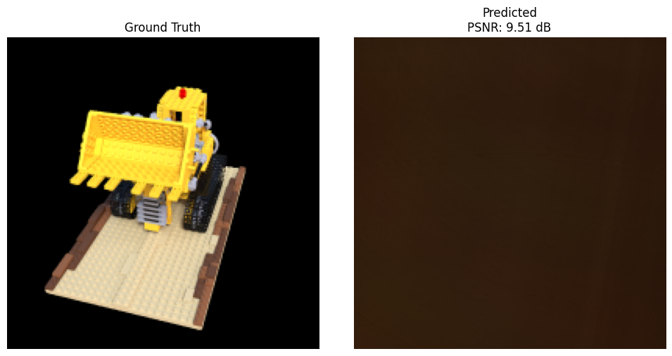
Part 2.6 Training with Your Own Data

The training data that I use is a doggy of mine. Here is the demonstration of the data: (The data is first resized to 200x200 for faster evaluation.)

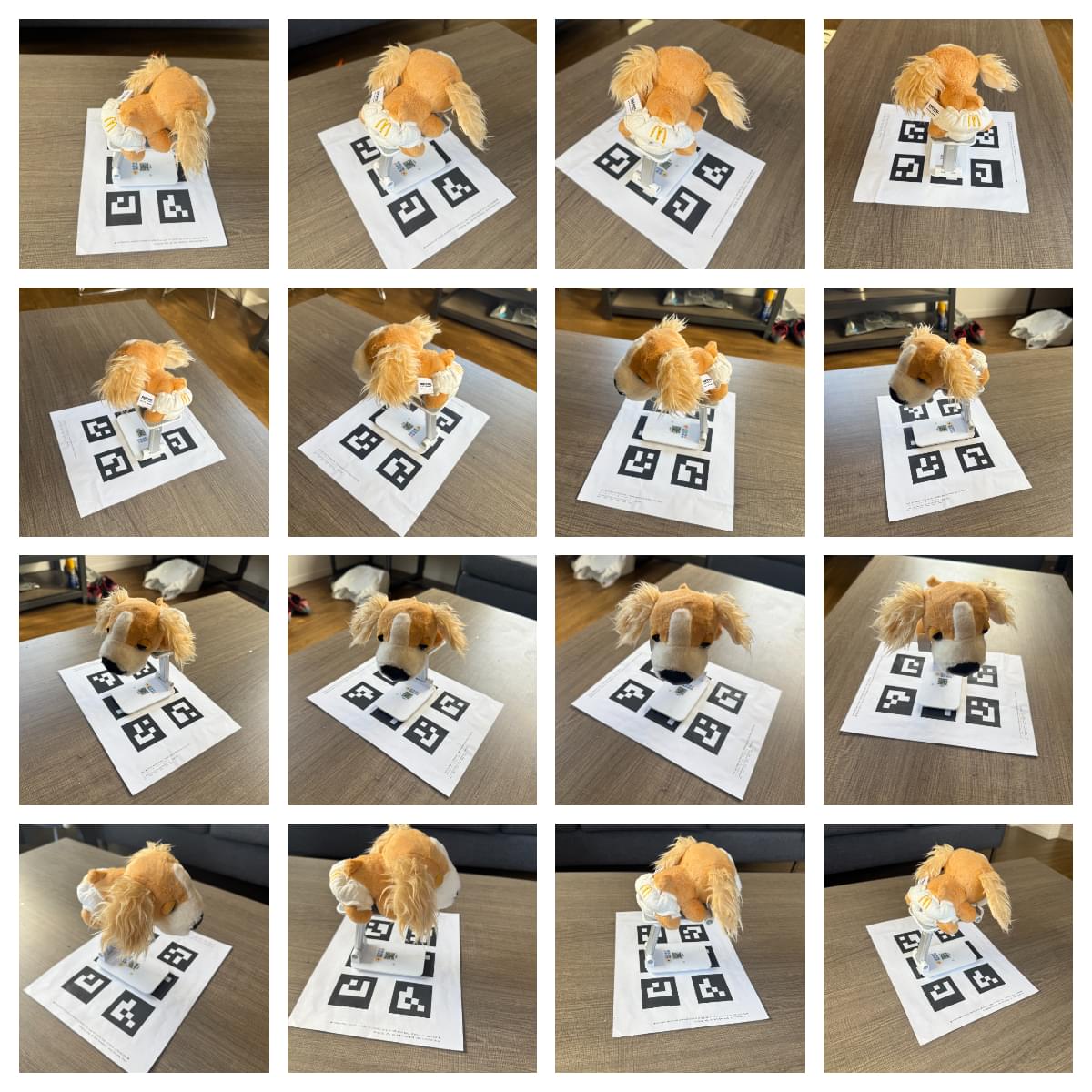
I have taken in total 38 images of the doggy from different angles and different distances. I try to keep the distance of the camera nearly the same for each image. After ArUco tags detection, only 29 images survive with having ID 4 tags in the image. Using the 28 of the images for training and the other 1 image for validation, I get the following results:

Test Video

Hyperparameter Tuning

Here I tune the hyperparameters of the model to get the best performance. I tune the following hyperparameters:

1. Sample near and far distance from the camera.
2. Sample num_samples number of points along the ray.
3. Training steps

These parameters are important as if we choose the distance too far, it has high possibility that those points are occluded and therefore do not contribute to the final color of the ray. Also, if we sample too few points, it will not be able to capture the details of the scene and will lead to some bad holes in the rendering.

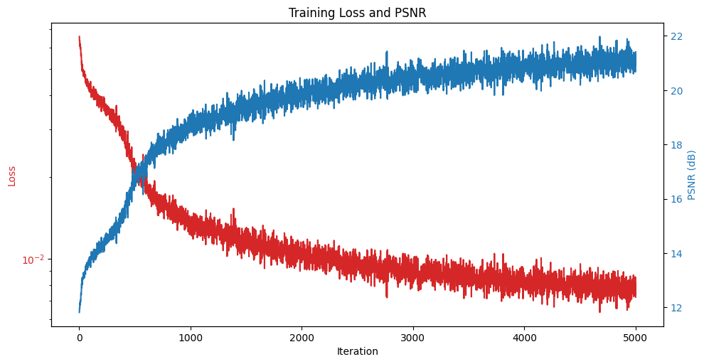
Training loss over iterations

Intermediate renders of the scene during training

Here are the intermediate renders of the scene during training. We can see that the model is able to fit the training data well.