Part A: The Power of Diffusion Models!

Part 0: Setup

Results Comparison: Different Resolutions and Inference Steps

The following table shows the generated images for 5 different prompts, comparing low resolution (after stage 1 of the network) vs high resolution (after stage 2 of the network), and 20 inference steps vs 50 inference steps.

Prompt	Low Resolution 20 Steps	Low Resolution 50 Steps	High Resolution 20 Steps	High Resolution 50 Steps
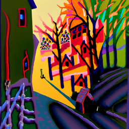
1. An oil painting of a snowy mountain village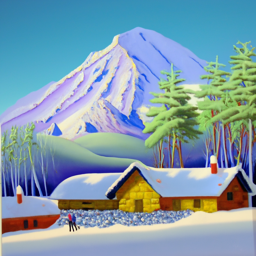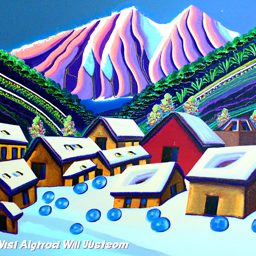
2. An oil painting of an old man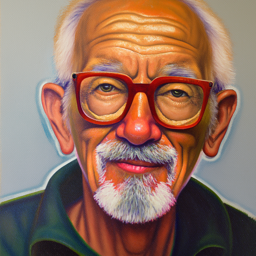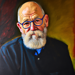
3. An oil painting of a young lady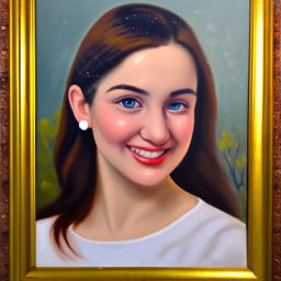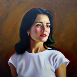
4. A lithograph of waterfalls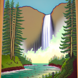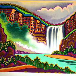
5. A lithograph of a skull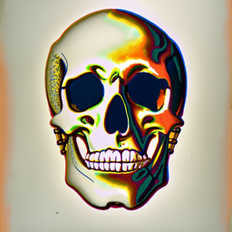

Analysis

This comparison demonstrates the effects of:

Resolution: High resolution images provide more detail and clarity compared to low resolution versions
Inference Steps: More inference steps (50 vs 20) generally result in more refined and detailed outputs, though the improvement may vary depending on the prompt (For example, for the two scenary views, the results in more inference steps do not look much better than the results in less inference steps, they seem both unrealistic.)

Part 1: Sampling Loops

Part 1.1 Implementing the Forward Process

The implementation of the forward function is as follows:

def forward(im, t):
    """
    Args:
        im : torch tensor of size (1, 3, 64, 64) representing the clean image
        t : integer timestep

    Returns:
        im_noisy : torch tensor of size (1, 3, 64, 64) representing the noisy image at timestep t
    """
    with torch.no_grad():
        noise = torch.randn_like(im)
        alphas_t = alphas_cumprod[t]
        im_noisy = im * torch.sqrt(alphas_t) + torch.sqrt(1 - alphas_t) * noise
    return im_noisy

Noise Level: 250

Noise Level: 500

Noise Level: 750

Original

Part 1.2 Classical Denoising

This section demonstrates the effect of traditional Gaussian blur denoising on noisy images. The images below show a comparison between the noisy images (before denoising) and the results after applying Gaussian blur denoising.

Noise Level	Before Denoising (Noisy Image)	After Gaussian Blur (Denoised Image)
Noise Level: 250
Noise Level: 500
Noise Level: 750
Original

The comparison above demonstrates the effect of Gaussian blur denoising:

Noise Reduction: Gaussian blur effectively reduces high-frequency noise, making the images appear smoother. While noise is reduced, Gaussian blur also tends to blur fine details and edges, resulting in a loss of sharpness
Limitations: Traditional Gaussian blur is a simple denoising method that doesn’t preserve image structure as well as more advanced denoising techniques like diffusion models

Part 1.3 Implementing One Step Denoising

The one step denoising is mainly by the following steps:

Use forward to get the noisy image at timestep t
Estimate the noise at timestep t
Remove the noise to get an estimate of the original image

Noise Level	Original Image	Before Denoising (Noisy Image)	After One Step Denoising (Denoised Image)
Noise Level: 250
Noise Level: 500
Noise Level: 750

Part 1.4 Implementing Iterative Denoising

The iterative denoising loop repeatedly applies our learned denoiser while walking backward through the noise schedule. Each pass removes the predicted noise for the current timestep and re-injects the correct level of randomness, giving the next, slightly cleaner image. Repeating this across many steps (rather than performing a single giant leap) preserves structure while gradually restoring finer details. The implementation of the iterative_denoising function is as follows:

def iterative_denoise(im_noisy, i_start, prompt_embeds, timesteps, display=True):
  image = im_noisy
  images_to_display = []

  with torch.no_grad():
    for i in range(i_start, len(timesteps) - 1):
      # Get timesteps
      t = timesteps[i]
      prev_t = timesteps[i+1]

      # get `alpha_cumprod` and `alpha_cumprod_prev` for timestep t from `alphas_cumprod`
      # compute `alpha`
      # compute `beta`
      # ===== your code here! =====
      alpha_cumprod = alphas_cumprod[t]
      alpha_cumprod_prev = alphas_cumprod[prev_t]
      alpha_t_step = alpha_cumprod / alpha_cumprod_prev
      beta_t_step = 1 - alpha_t_step
      # ==== end of code ====

      # Get noise estimate
      model_output = stage_1.unet(
          image.half().cuda(),
          t,
          encoder_hidden_states=prompt_embeds,
          return_dict=False
      )[0]

      # Split estimate into noise and variance estimate
      noise_est, predicted_variance = torch.split(model_output, image.shape[1], dim=1)

      # compute `pred_prev_image` (x_{t'}), the DDPM estimate for the image at the
      # next timestep, which is slightly less noisy. Use the equation 3.
      # This is the core of DDPM
      # ===== your code here! =====
      x0_pred = (image - torch.sqrt(1 - alpha_cumprod) * noise_est) / torch.sqrt(alpha_cumprod)

      # Apply equation 3
      pred_prev_image = (
          (torch.sqrt(alpha_cumprod_prev) * beta_t_step / (1 - alpha_cumprod)) * x0_pred +
          (torch.sqrt(alpha_t_step) * (1 - alpha_cumprod_prev) / (1 - alpha_cumprod)) * image
      )
      pred_prev_image = add_variance(predicted_variance, t, pred_prev_image)

      if t in [90, 240, 390, 540, 690]:
        iterative_images[t] = (pred_prev_image.squeeze(0) * 0.5 + 0.5).clamp(0, 1).cpu().numpy().transpose(1, 2, 0)

      # ==== end of code ====

      image = pred_prev_image

    clean = image.cpu().detach().numpy()
  return clean

Original	Gaussian Blur	One-Step Denoising	Iterative Denoising

Noise Level: 690

The slider highlights how the sample becomes progressively clearer as we move from heavy noise (690) toward the final reconstruction. The gradual refinement with multiple steps avoids the over-smoothing artifacts seen in the Gaussian blur and produces noticeably sharper edges than the single-step approach.

Part 1.5 Diffusion Model Sampling

The full sampling loop produces high-quality generations from pure noise. Below are five samples (using the same prompt embeddings from ‘a high quality photo’) captured at the final timestep of the iterative procedure:

Sample 1

Sample 2

Sample 3

Sample 4

Sample 5

Part 1.6 Classifier-Free Guidance (CFG)

I implement the iterative_denoise_cfg function to add classifier-free guidance to the iterative denoising process. The implementation is as follows:

def iterative_denoise_cfg(im_noisy, i_start, prompt_embeds, uncond_prompt_embeds, timesteps, scale=7):
  image = im_noisy
  images_to_display = []

  with torch.no_grad():
    for i in range(i_start, len(timesteps) - 1):
      # Get timesteps
      t = timesteps[i]
      prev_t = timesteps[i+1]

      # Get `alpha_cumprod`, `alpha_cumprod_prev`, `alpha`, `beta`
      # ===== your code here! =====
      alpha_cumprod = alphas_cumprod[t]
      alpha_cumprod_prev = alphas_cumprod[prev_t]
      alpha_t_step = alpha_cumprod / alpha_cumprod_prev # This is alpha_t in equation 3
      beta_t_step = 1 - alpha_t_step # This is beta_t in equation 3
      # ==== end of code ====

      # Get cond noise estimate
      model_output = stage_1.unet(
          image,
          t,
          encoder_hidden_states=prompt_embeds,
          return_dict=False
      )[0]

      # Get uncond noise estimate
      uncond_model_output = stage_1.unet(
          image,
          t,
          encoder_hidden_states=uncond_prompt_embeds,
          return_dict=False
      )[0]

      # Split estimate into noise and variance estimate
      noise_est, predicted_variance = torch.split(model_output, image.shape[1], dim=1)
      uncond_noise_est, _ = torch.split(uncond_model_output, image.shape[1], dim=1)

      # Compute the CFG noise estimate based on equation 4
      # ===== your code here! =====
      noise_est_cfg = uncond_noise_est + scale * (noise_est - uncond_noise_est)
      # ==== end of code ====


      # Get `pred_prev_image`, the next less noisy image.
      # Predict x0 using the CFG noise estimate
      # ===== your code here! =====
      x0_pred = (image - torch.sqrt(1 - alpha_cumprod) * noise_est_cfg) / torch.sqrt(alpha_cumprod)

      # Apply equation 3
      pred_prev_image = (
          (torch.sqrt(alpha_cumprod_prev) * beta_t_step / (1 - alpha_cumprod)) * x0_pred +
          (torch.sqrt(alpha_t_step) * (1 - alpha_cumprod_prev) / (1 - alpha_cumprod)) * image
      )
      pred_prev_image = add_variance(predicted_variance, t, pred_prev_image)
      # ==== end of code ====

      image = pred_prev_image

    clean = image.cpu().detach().numpy()
  return clean

The following images show the results of the iterative denoising with CFG:

Sample 1

Sample 2

Sample 3

Sample 4

Sample 5

Part 1.7 Image-to-image Translation

We now explore how strongly the diffusion process can pull a slightly corrupted real image back to the learned image manifold when we start the reverse process at different points in the noise schedule. I add a small amount of noise to the Campanile photo, then jump into the sampler at indices [1, 3, 5, 7, 10, 20] (the indices correspond to positions within the noise schedule; smaller values mean we restart from a noisier state and therefore denoise over a longer trajectory).

Start @ 1

Start @ 3

Start @ 5

Start @ 7

Start @ 10

Start @ 20

Original

Part 1.7.1 Editing Hand-Drawn and Web Images

In this section, we will use pictures from the web and hand-drawn images to test the editing ability of the diffusion model.

Start @ 1

Start @ 3

Start @ 5

Start @ 7

Start @ 10

Start @ 20

Original

Part 1.7.2 Inpainting

In this section, we will use the inpainting method to fill in the missing parts of the images. The technique is to only allow denoising in the masked region and keep the rest of the image unchanged.

Original Image

Mask Image

Replace Area

Result Image

Part 1.7.3 Text-Conditioned Image-to-image Translation

In this section, we change the prompt ‘A high quality photo’ to my own prompt and see the translation results. The technique is to use pictures with similar structure, or the translation process will not be smooth.

Start @ 1

Start @ 3

Start @ 5

Start @ 7

Start @ 10

Start @ 20

Original

Part 1.8 Visual Anagrams

In this section, we will use the visual anagrams method to create a new image from the original images. The visual anagrams are created using the following steps:

$\epsilon_1 = \text{CFG of UNet}(x_t, t, p_1)$
$\epsilon_2 = \text{flip}(\text{CFG of UNet}(\text{flip}(x_t), t, p_2))$
$\epsilon = (\epsilon_1 + \epsilon_2) / 2$

where UNet is the diffusion model UNet from before, $\text{flip}(\cdot)$ is a function that flips the image, and $p_1$ and $p_2$ are two different text prompt embeddings.

An oil painting of an old man
↔
An oil painting of an young lady

Click to flip

An oil painting of a snowy mountain village
↔
An oil painting of people around a campfire

Click to flip

Part 1.9 Hybrid Images

For the Hybrid Images, we are taking the low-pass noise of the first image and the high-pass noise of the second image and then add them together to get the hybrid image. The algorithm is as follows:

$\epsilon_1 = \text{CFG of UNet}(x_t, t, p_1)$
$\epsilon_2 = \text{CFG of UNet}(x_t, t, p_2)$
$\epsilon = f_\text{lowpass}(\epsilon_1) + f_\text{highpass}(\epsilon_2)$

where UNet is the diffusion model UNet, $f_\text{lowpass}$ is a low pass function, $f_\text{highpass}$ is a high pass function, and $p_1$ and $p_2$ are two different text prompt embeddings. Our final noise estimate is $\epsilon$ .

The following are the results of the hybrid images:

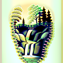
A lithograph of a skull
↔
A lithograph of waterfalls

High Pass (Normal Picture)

A painting of a red panda
↔
A painting of houseplant

High Pass (Normal Picture)

Part B: Flow Matching from Scratch

Part 1: Training a Single-Step Denoising UNet

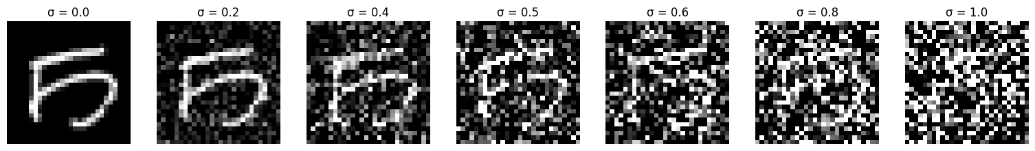
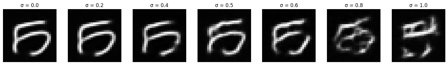
Visualization of the Noising process

After implementing the UNet, we can visualize the noising process by selecting different noise levels $\sigma$ . The following are the results of the noising process:

Noising process with different noise levels

Training Process Visualization

I have trained the UNet for 5 epochs and each epoch process 253 batches with the batch size of 64. I select some of the images in the batch and produce a visualization of the training process. The following are the results before the training (epoch 0) and after the training (epoch 5):

Before Training (Epoch 0)

After Training (Epoch 5)

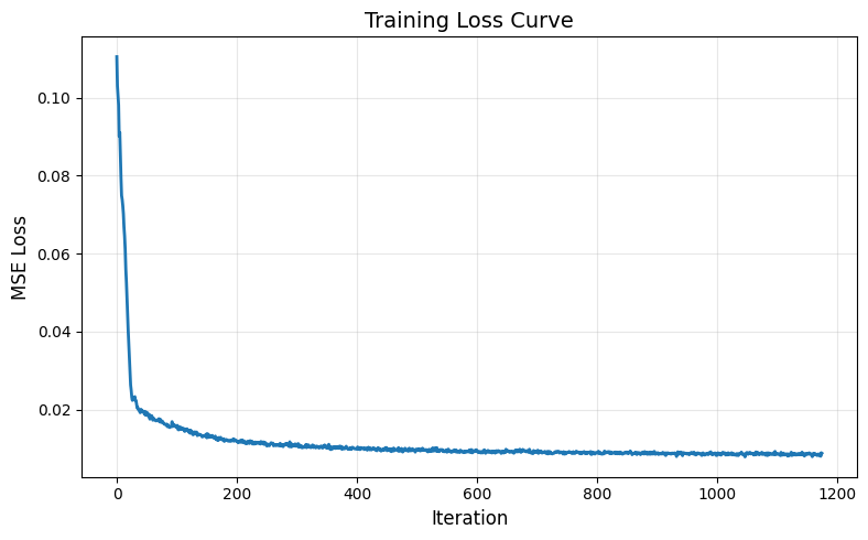
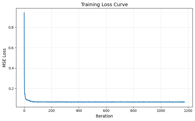
Training Loss Visualization

The training loss is as follows:

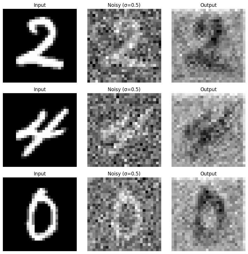
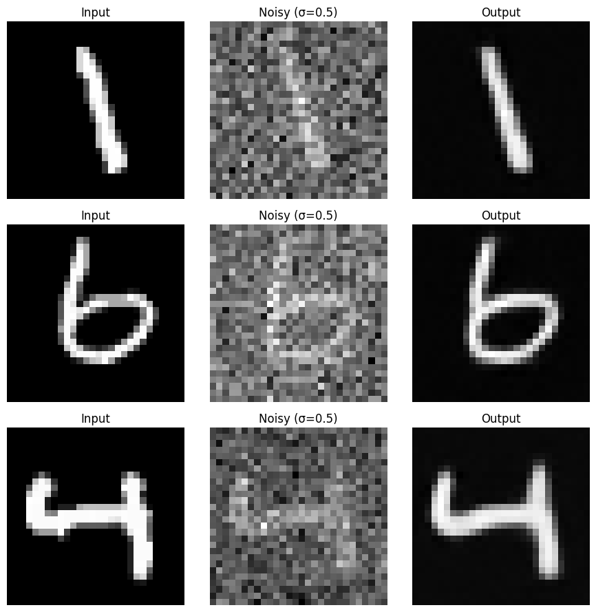
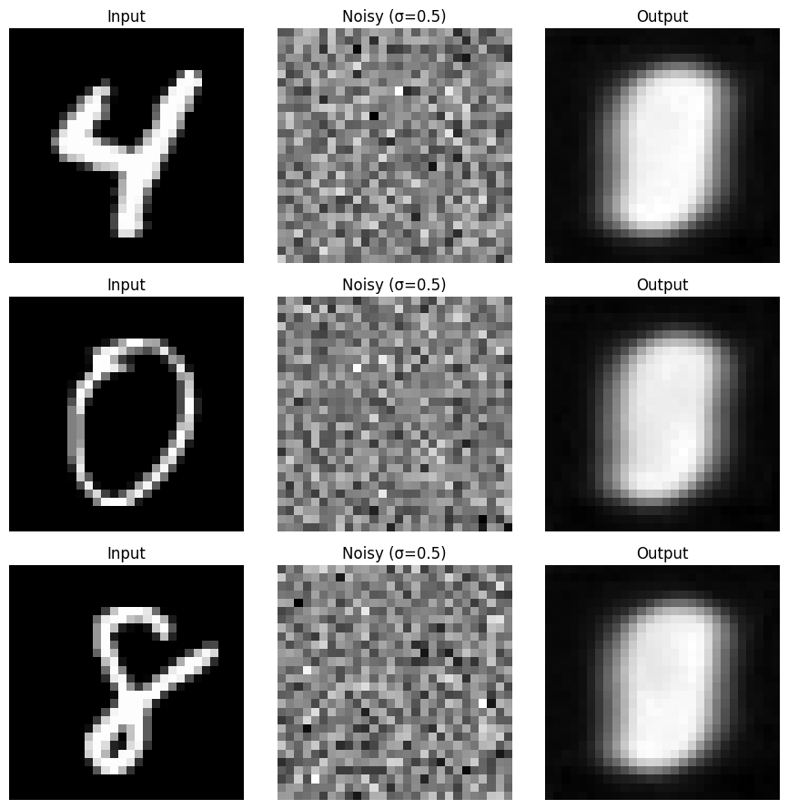
Out-of-Distribution Testing

I sample results on the test set with out-of-distribution noise levels after the model is trained. The following are the results:

You can see that for the noise level that was lower than 0.5, the generated images are quite good. However, for the noise level that was higher than 0.5, the denoised images perform poorly. This is because the model is not adapted to the noise higher than 0.5.

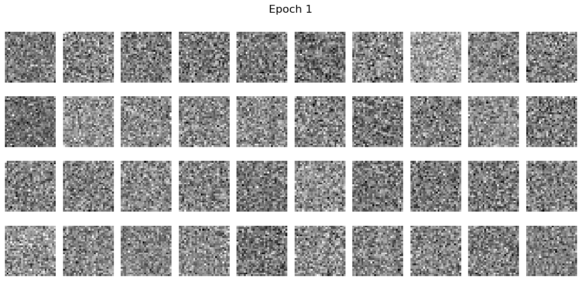
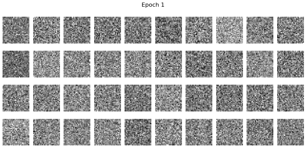
Denoising Pure Noise Visualization

I used the trained model to denoise pure noise (input the pure noise and then use the images to calculated the mean as loss) and the visualization of the training process are as follows:

Before Training (Epoch 0)

After Training (Epoch 5)

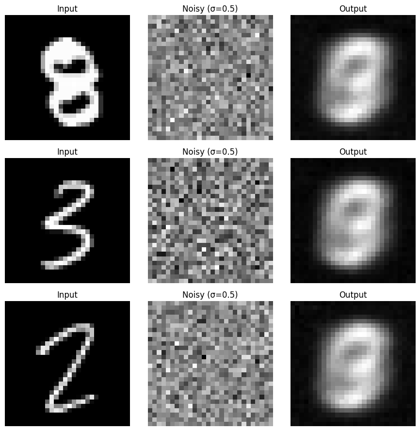
You can see that the model can barely denoise the pure noise.

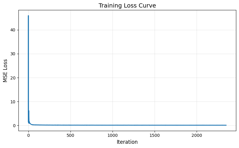
Denoising Pure Noise Training Loss Visualization

The training loss is as follows:

The training loss is decreasing, however the results for different labels are the same. This is because when we train the model using pure noise as input, the model cannot distinguish the differences between the inputs of different labels. Thus, the results for all the predicted labels are very similar because they are trained on a dataset that does not really distinguish the input. So the results seem to be a combination of all the numbers, you can see a ‘3’ shape, ‘6’ shape and ‘8’ shape because there are overlapping curves for these numbers. The results can also be summarized as a centroid for all the shape of the numbers.

Part 2: Training a Flow Matching Model

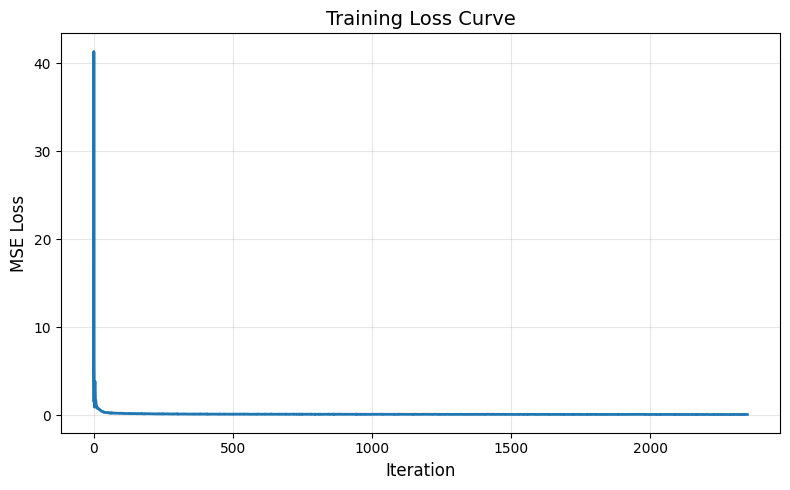
Training Loss for Time-Contiditioned UNet

After implementing the UNet as told in the ipynb notebook and the tutorial, I was able to train the flow matching model with converging loss. The learning rate I use is $1e-2$ and the $\gamma$ for the scheduler is $0.99$ .

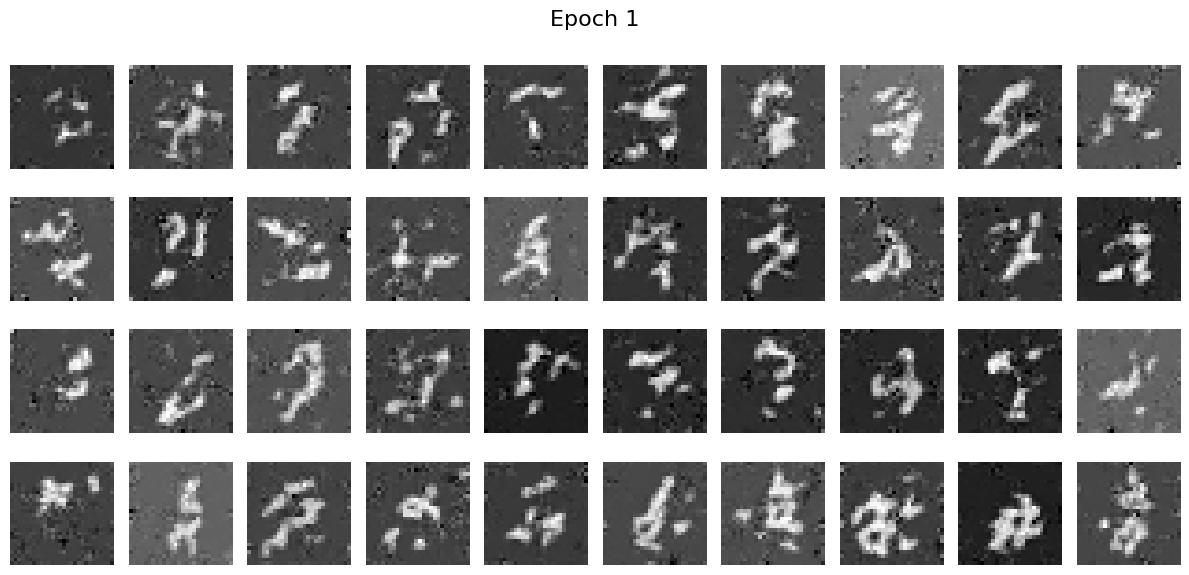
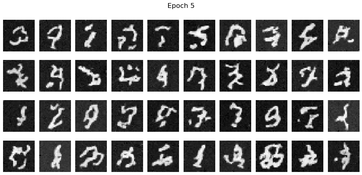
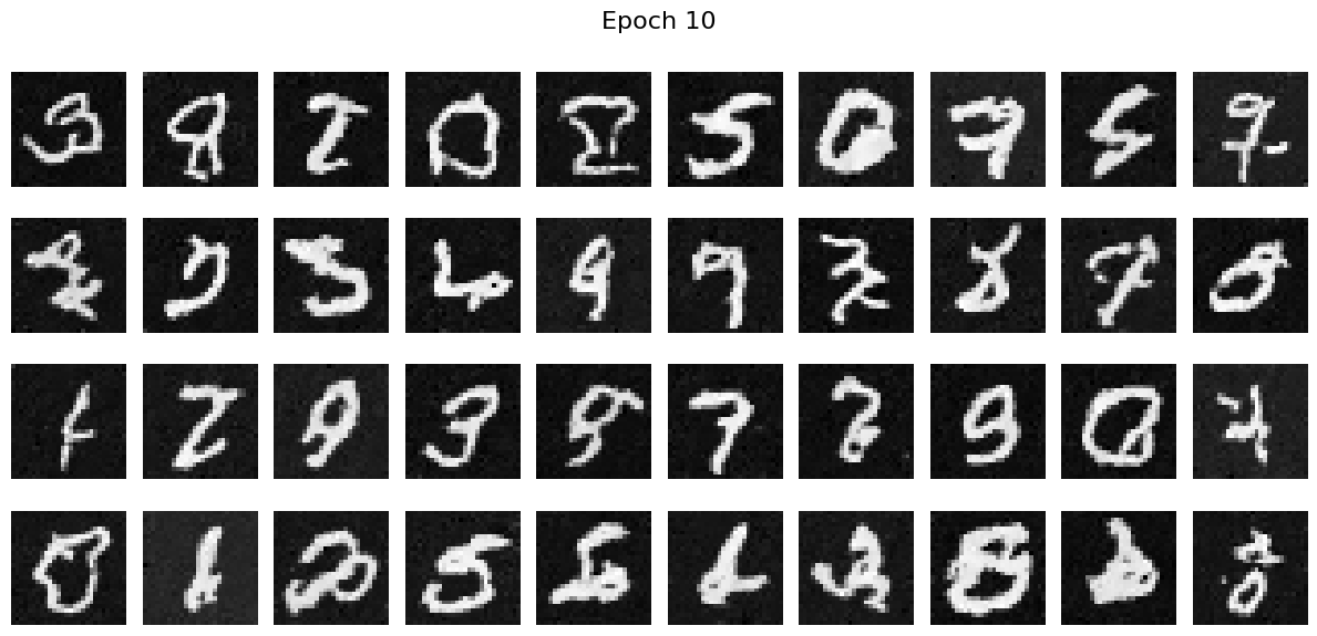
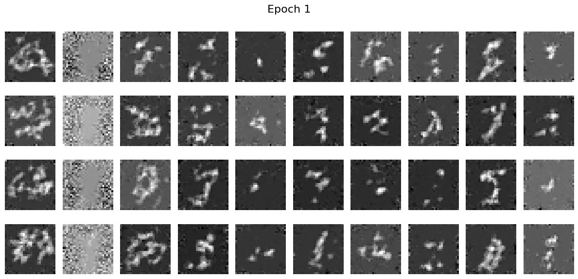
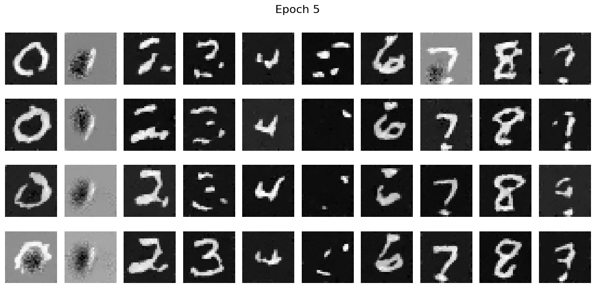
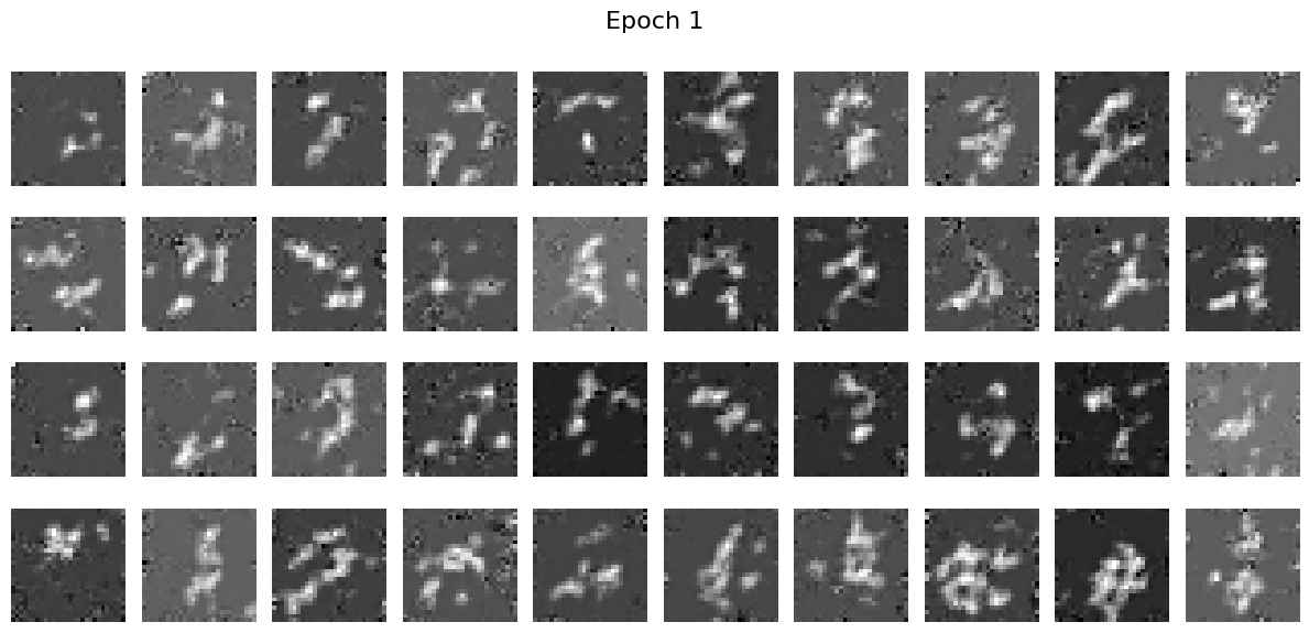
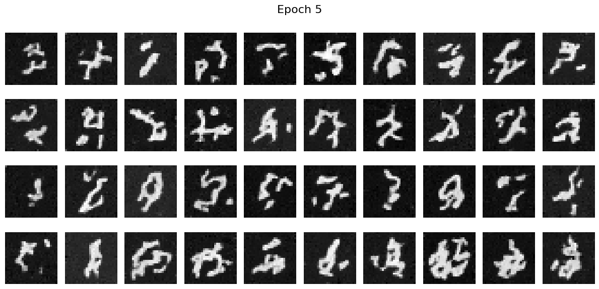
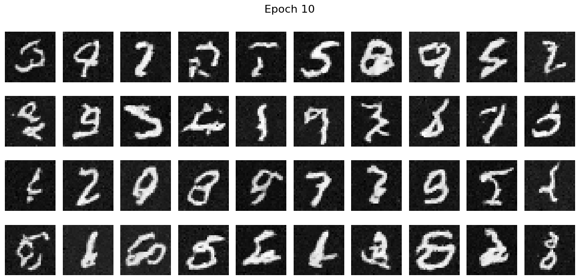
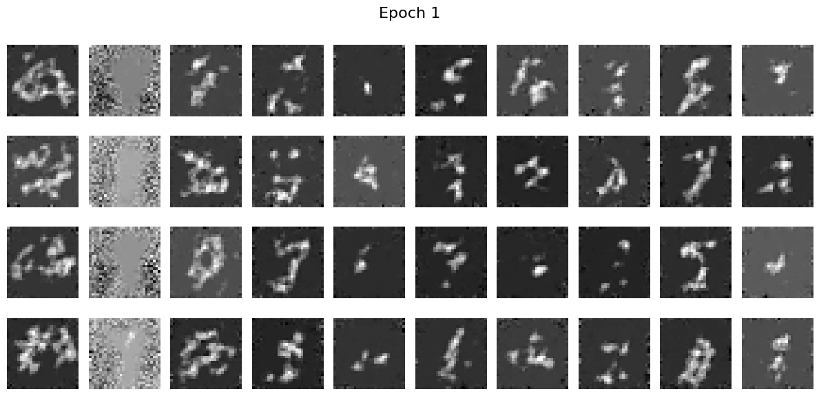
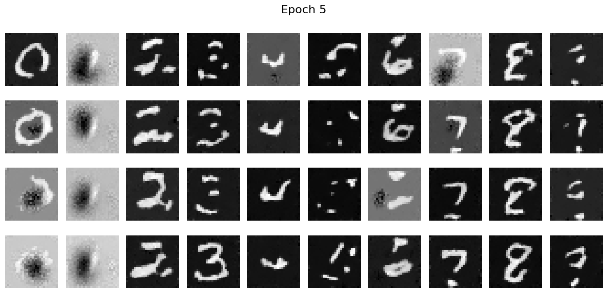
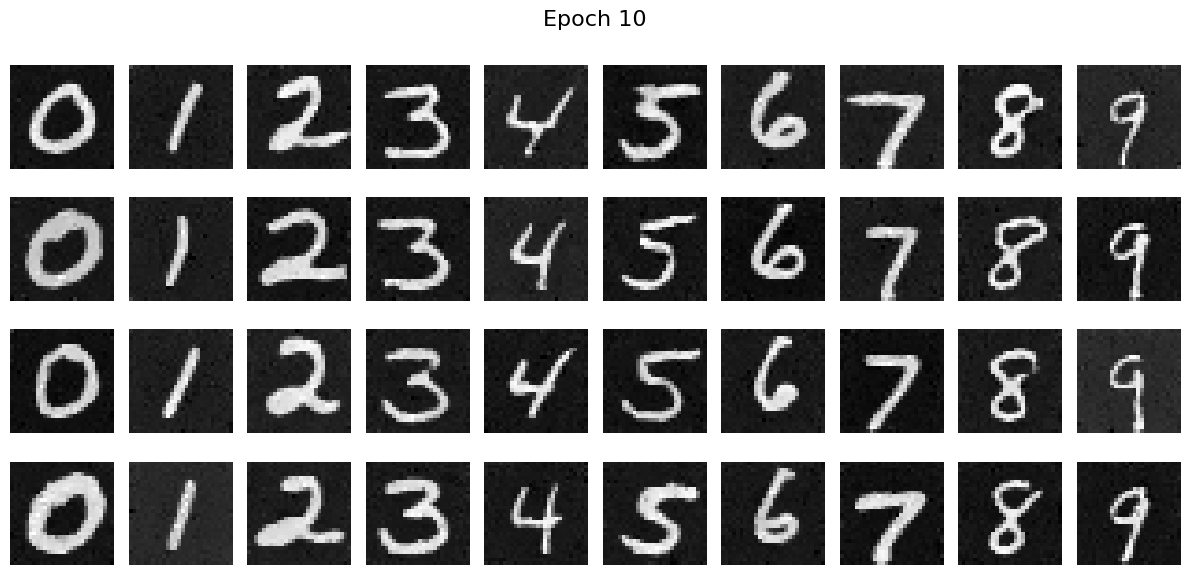
Sampling results from the Time-Conditioned UNet

I sampled some results from the epoch 1, 5 and 10 and we can see that the resuls are quite good.

Before Training (Epoch 0)

After Epoch 1

After Epoch 5

After Epoch 10

Training Loss for Class-Conditioned UNet

Using the same parameters in the Time-Conditioned UNet, we can get the following training curve.

Sampling results from the Class-Conditioned UNet

The visulization results are as follows:

Before Training (Epoch 0)

After Epoch 1

After Epoch 5

After Epoch 10

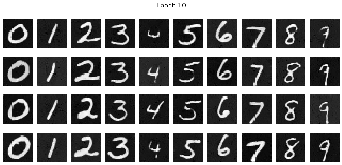
We can see that the Class-Conditioned UNet can help generate more accurate and clearer results than the time-conditioned network.

Train without scheduler

We observe that train without scheduler does not directly lead to a bad results. However, it does lead to slower convergence and therefore it is better to use scheduler.

Results with Time-Conditioned Network:

Before Training (Epoch 0)

After Epoch 1

After Epoch 5

After Epoch 10

Results with Class-Conditioned Network:

Before Training (Epoch 0)

After Epoch 1

After Epoch 5

After Epoch 10

We can see that the differences between using scheduler and not using shceduler are not huge. However, using scheduler does lead to faster convergence.